Coordination, Components, and Cloud

EE 547 - Unit 1

Dr. Brandon Franzke

Spring 2026

Coordination in Computing

Distributed Systems Span Multiple Machines

A web application in production:

Load balancer receives requests
Application servers process business logic
Database stores persistent state
Cache holds frequently-accessed data
Background workers handle async tasks

Each component runs as a separate process, often on separate machines. No component can directly access another’s memory.

This is the norm for modern applications. The single-machine program is the exception, not the rule.

Components Communicate Through Messages

When the application server needs user data, it cannot read the database’s memory. It sends a request and waits for a response.

App Server                    Database
    |                            |
    |-------- request --------->|
    |                            |
    |         (processing)       |
    |                            |
    |<------- response ---------|
    |                            |

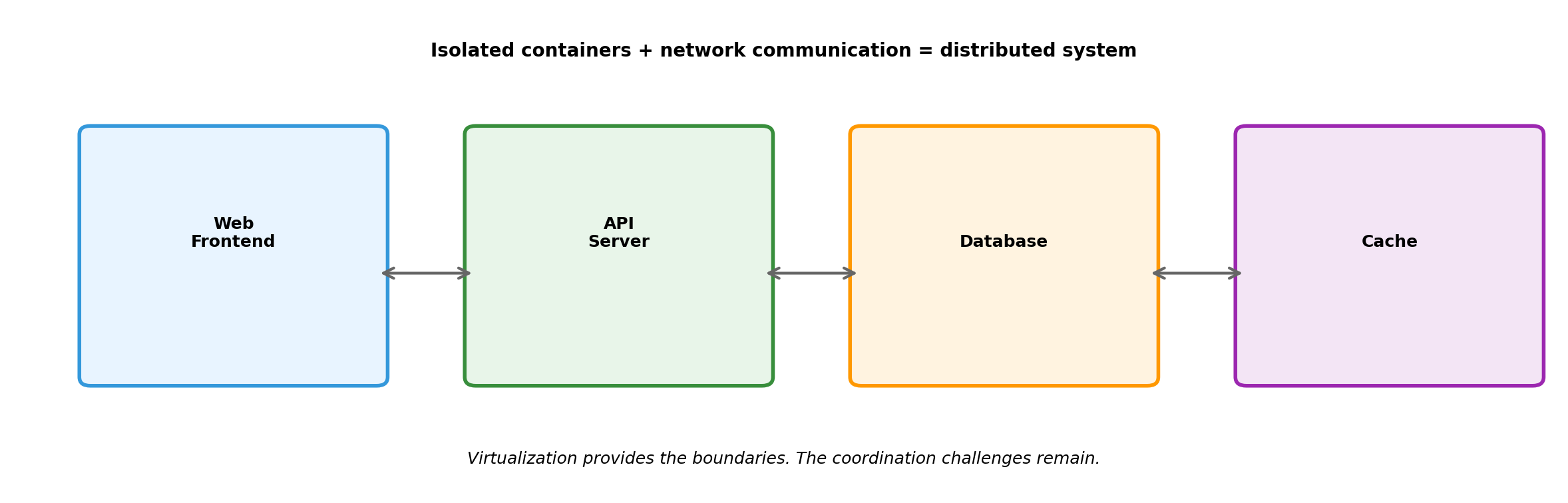
Every interaction between components follows this pattern. Query results, cache lookups, API calls—all require explicit message exchange.

The application server’s code pauses, waiting for bytes to arrive over the network.

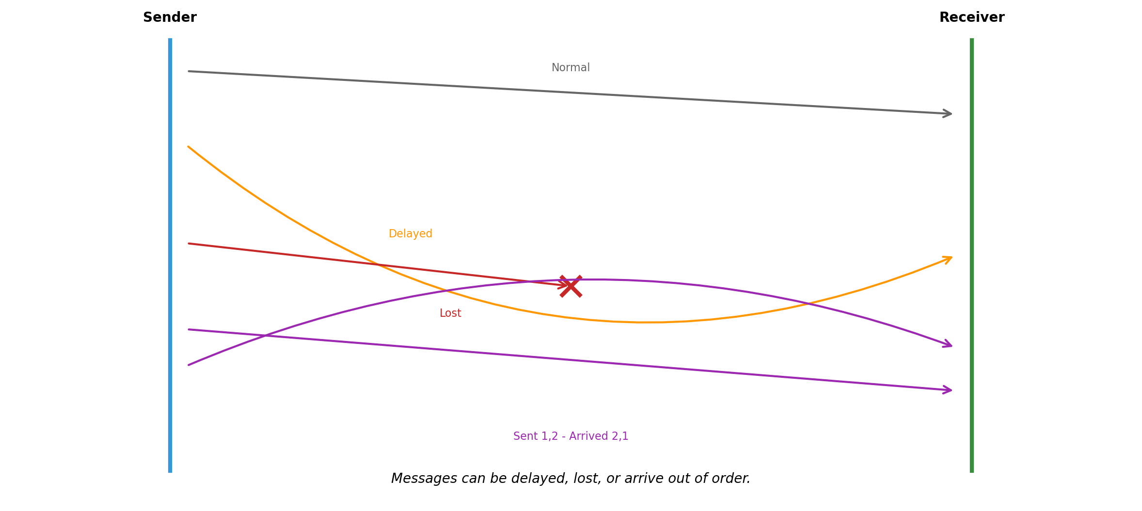
Messages Can Be Lost, Delayed, or Reordered

The network is not a function call. When the app server sends a query:

The request might not arrive. Router failure, network partition, packet corruption.

The request might arrive late. Congestion, retransmission, routing changes.

The response might not arrive. Database processed the query, but the response was lost.

Messages might arrive out of order. Request A sent before B, but B arrives first.

None of these failure modes exist in a single process. A function call either executes or the process crashes. There is no “maybe it executed.”

A Request Without Response Creates Uncertainty

A function call has two outcomes: return a value, or throw an exception. A network request has three.

Success

Request sent. Server processed. Response received.

Client knows the operation completed.

result = db.query(sql)
# result contains data

Failure

Request sent. Server returned error. Error received.

Client knows it failed.

try:
    result = db.query(sql)
except DatabaseError:
    # handle known failure

Unknown

Request sent. No response.

Did the server receive it? Process it? Crash before? After?

try:
    result = db.query(sql)
except Timeout:
    # did it succeed or not?

The unknown case forces difficult decisions. Retry and risk duplicate execution. Don’t retry and risk losing the operation.

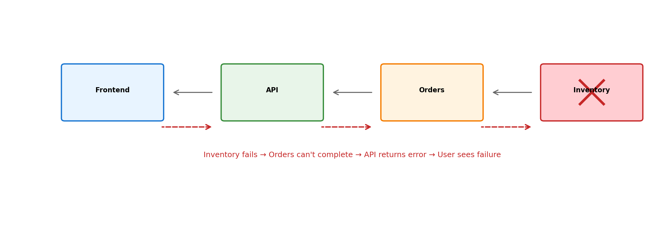
Partial Failure: Some Components Work While Others Don’t

A single-machine program either runs or doesn’t. A distributed system occupies states in between.

Some requests succeed. Others fail. Others succeed slowly. The outcome depends on which path a request takes through the system.

Every component must be written assuming the components it depends on might be unavailable—right now, for this request, even if they worked a moment ago.

No Global Clock Orders Events

Machine A’s clock: 10:00:00.000

Machine B’s clock: 10:00:00.003

A sends a message at its 10:00:00.000. B receives it at its 10:00:00.002.

Meanwhile, B had a local event at its 10:00:00.001.

Did A’s send happen before or after B’s event? The timestamps suggest A sent first (10:00:00.000 < 10:00:00.001), but A’s clock might be behind B’s.

Clocks drift. Synchronization protocols get them close—milliseconds—but not identical. For operations that happen within milliseconds of each other, timestamps cannot determine order.

In a single process, “before” means “earlier in the instruction sequence.” Across machines, there is no shared instruction sequence to consult.

These Challenges Seem Fundamental to Distribution

No shared memory. Network uncertainty. Partial failure. No global clock.

These arise because components run on separate machines, communicating over a network.

But consider: are these really about the network? Or about something more fundamental?

A useful test: what if we remove the network?

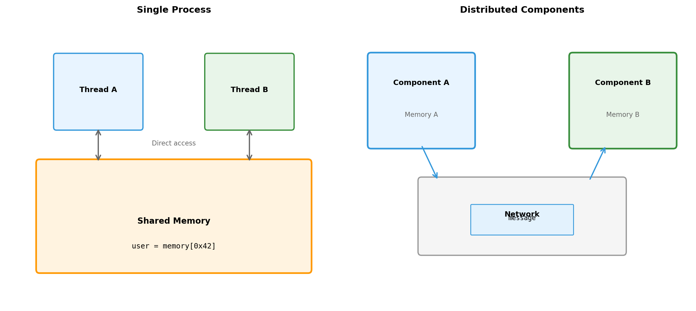
A Single Process Has Implicit Coordination

total = 0
for item in items:
    total += item.price
print(f"Total: ${total}")

Each statement executes after the previous completes.

The variable total exists in one place. Reading it returns what was last written.

If the loop crashes, the entire process stops. No ambiguity about what state persists.

These properties require no effort from the programmer. The language runtime provides them automatically.

One thread of execution. Shared memory. Single failure domain. Coordination is implicit.

A Thread Is an Independent Execution Context Within a Process

A process can contain multiple threads. Each thread:

Has its own instruction pointer (where it is in the code)
Has its own stack (local variables, function calls)
Shares the process’s memory (global variables, heap)
Runs concurrently with other threads

The operating system schedules threads, switching between them. From each thread’s perspective, it runs continuously. In reality, threads interleave.

Threads enable parallelism within a process. Multiple CPU cores can execute different threads simultaneously. A web server might handle each request in a separate thread.

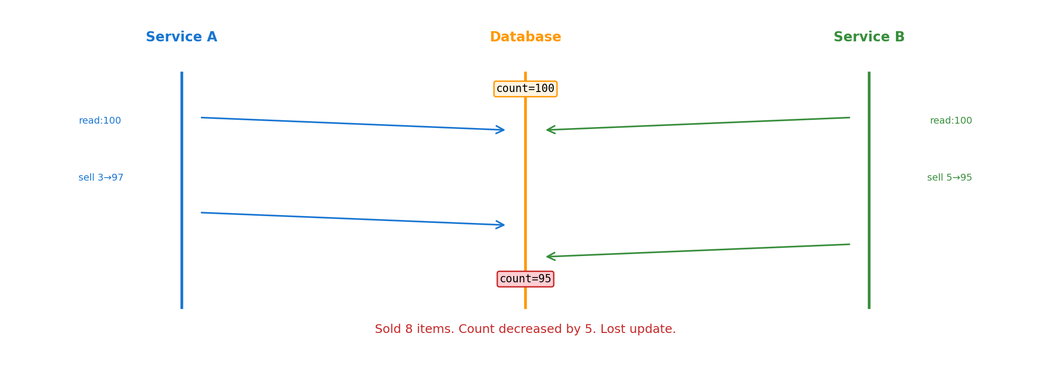
Two Threads Sharing State Require Explicit Coordination

# Shared state
total = 100

# Thread A              # Thread B
read total  → 100       read total  → 100
add 50      → 150       add 30      → 130
write total ← 150       write total ← 130

Both threads read total = 100. Thread A computes 150, Thread B computes 130. Whichever writes last wins.

Expected result: 180.

Actual result: 130 or 150.

Both threads run on the same CPU. Memory access takes nanoseconds. The problem is not speed. Two agents modified shared state without coordination.

Threading Bugs Occur Without Any Network

Deadlock: Two locks, opposite order

# Thread A              # Thread B
acquire(lock_1)         acquire(lock_2)
acquire(lock_2)  ←wait  acquire(lock_1)  ←wait

Thread A holds lock_1, waits for lock_2. Thread B holds lock_2, waits for lock_1. Neither proceeds.

Lost update: Check-then-act

if count > 0:
    # Thread B decrements count here
    count -= 1  # Now negative

Visibility: Cached state

Thread A writes flag = True. Thread B reads flag = False. Each thread’s view of memory differs due to CPU caching.

These are coordination failures. No network involved. Shared memory. Nanosecond access. Still broken.

Coordination Difficulty Is Not About Speed

Threading demonstrates the point: coordination challenges exist even when:

Memory is shared (no messages needed)
Access is fast (nanoseconds, not milliseconds)
Failure is atomic (whole process crashes, no partial failure)
There’s a global clock (CPU timestamp counter)

The difficulty is reasoning about concurrent access to shared state. Multiple agents, acting independently, can interfere with each other.

Adding network distribution makes coordination harder—but it doesn’t create the fundamental problem. The fundamental problem is concurrency itself.

Distribution amplifies coordination challenges. It doesn’t invent them.

Distribution Amplifies Every Coordination Challenge

Threads have:

Shared memory (can read each other’s state)

Same clock (CPU timestamp counter)

Atomic failure (process crashes entirely)

Synchronous primitives (locks, semaphores)

Distributed components have:

No shared memory (must send messages)

No common clock (clocks drift independently)

Partial failure (some components fail, others continue)

Only asynchronous messages (no global locks)

Network Uncertainty Has No Threading Equivalent

When Thread A calls a function, the function executes or the process crashes. There is no intermediate state.

When Component A sends a message to Component B:

The message might never arrive. A could wait forever.

B might process the message and crash before responding. A doesn’t know if the operation succeeded.

B might be slow. A cannot distinguish “slow” from “dead.”

A times out and retries. But B processed the first request. Now the operation happens twice.

This uncertainty—not knowing whether a remote operation succeeded—has no equivalent in local programming. It requires fundamentally different patterns.

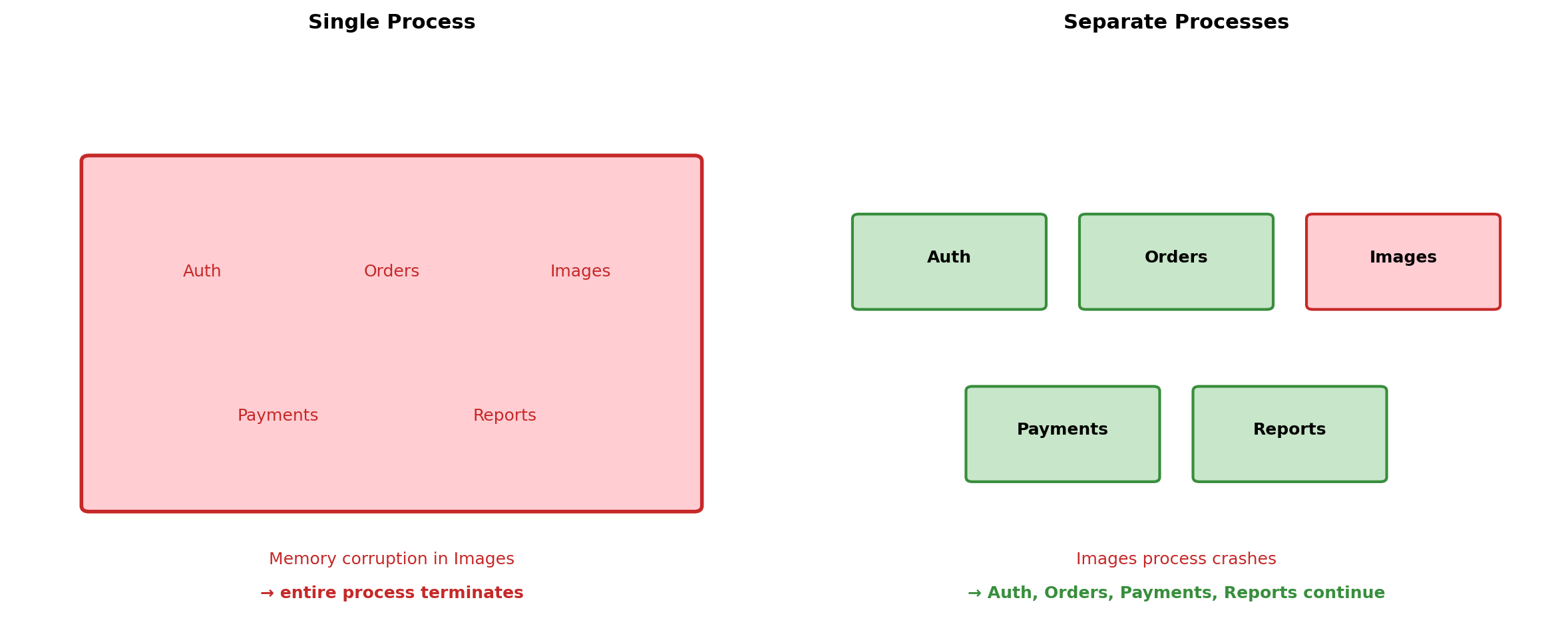
Partial Failure Has No Threading Equivalent

In a single process, failure is total. If any thread causes a segmentation fault, the entire process terminates. All threads die together.

In a distributed system, failure is partial. The database crashes. The web server continues running. It sends queries into a void and waits for responses that will never come.

Partial failure means:

Any component can fail at any time
Other components continue operating
Failed component might recover
Might recover with different state
Might never recover

Every component must handle the ongoing uncertainty of whether its dependencies are available, right now, for this operation.

These Challenges Exist at Every Scale

Two containers on a laptop. Two services in a datacenter. Two thousand instances across regions.

Web app calling a database

Application sends INSERT. Connection drops.

Did the INSERT succeed?
Retry might create duplicate row
No retry might lose the write

This happens whether the database is on the same machine, in the same rack, or across the world. The uncertainty is identical.

Background worker processing jobs

Worker pulls job from queue. Worker crashes.

Did it finish processing?
Should queue re-deliver?
Re-delivery might duplicate work
No re-delivery might lose the job

Same coordination problem at any scale. The number of machines changes the probability of failure, not the nature of it.

The patterns for handling uncertainty at small scale are the same patterns used at large scale.

Local Development Can Replicate Production Patterns

If coordination challenges were only about scale, you’d need a datacenter to learn distributed systems.

But the challenges are about structure, not size. A laptop running containers exhibits:

Network communication between components
Message loss and timeout scenarios
Independent component failure
State coordination across processes

The same architectural patterns apply. The same failure modes appear. The same solutions work.

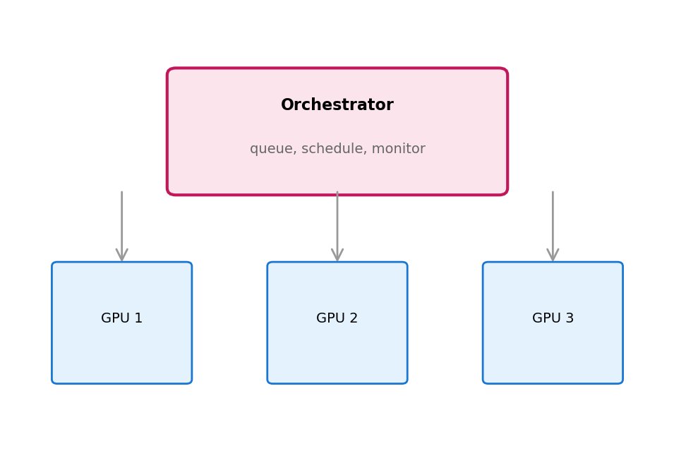
Course Topics Address Coordination Challenges

Isolation and packaging

Containers provide boundaries where components can fail independently. Orchestration manages component lifecycle.

Communication

APIs and protocols define how components exchange messages. HTTP, REST, and other patterns structure coordination.

State management

Databases provide coordination mechanisms for shared state. Storage systems handle persistence across failures.

Handling uncertainty

Timeouts, retries, and error handling manage the unknown outcomes of remote operations.

Composition

Services combine into systems where coordination requirements are explicit in the architecture.

Observability

Monitoring and logging make distributed behavior visible. Cannot attach a debugger across twelve machines.

Distribution creates coordination challenges. The course teaches patterns for managing them.

Why Distribute?

Distribution Adds Complexity

Coordination across components requires:

Explicit message passing instead of shared memory
Handling unknown outcomes from network requests
Designing for partial failure
Reasoning about ordering without a global clock

A single process avoids all of this. The runtime handles coordination implicitly.

Given the added complexity, distribution requires justification. What do separate components provide that a single process cannot?

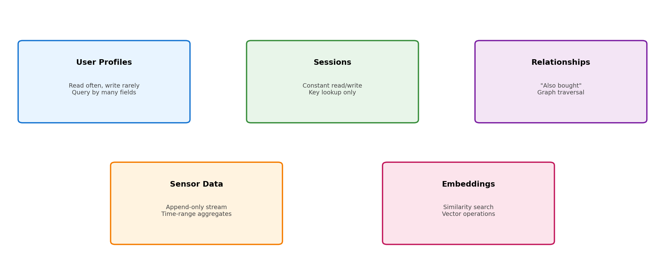
Specialized Components Optimize for Different Workloads

A database engine optimizes for:

Storage layouts that minimize disk seeks
Query planning across indexes
Transaction isolation between concurrent operations
Write-ahead logging for crash recovery

An HTTP server optimizes for:

Connection handling across thousands of clients
Request parsing and routing
Response streaming
TLS termination

Building both into one program means neither reaches its potential. Separate components allow focused optimization.

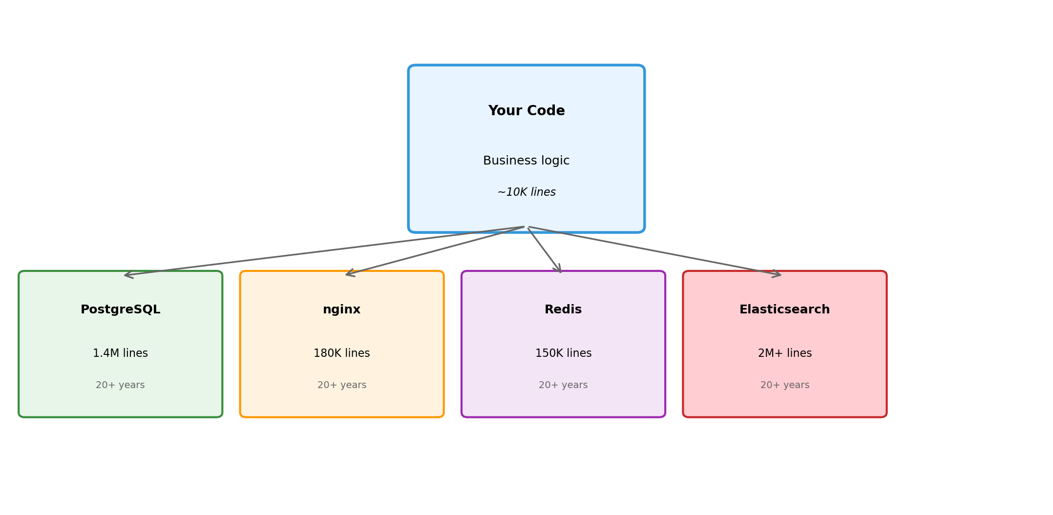
Years of Engineering Accumulate in Specialized Systems

PostgreSQL: first released 1996. Continuous development since then.

Query optimizer handles hundreds of plan variations
Storage engine manages page layout, TOAST, vacuuming
Replication supports streaming, logical, synchronous modes
Extensions enable custom types, indexes, languages

Replicating this in application code: impractical. The specialization represents decades of focused work on a specific domain.

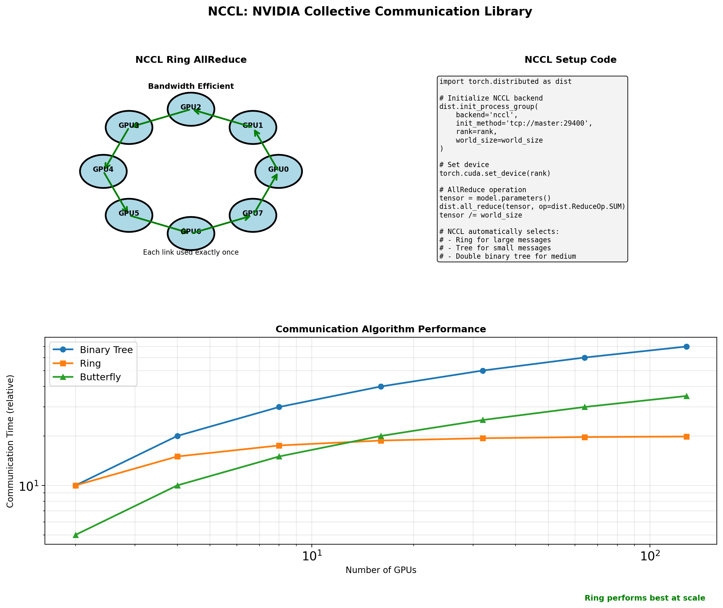
The same applies to web servers (nginx, Apache), caches (Redis, Memcached), message queues (RabbitMQ, Kafka), search engines (Elasticsearch), and every other infrastructure component.

Using specialized components means building on accumulated expertise rather than starting from scratch.

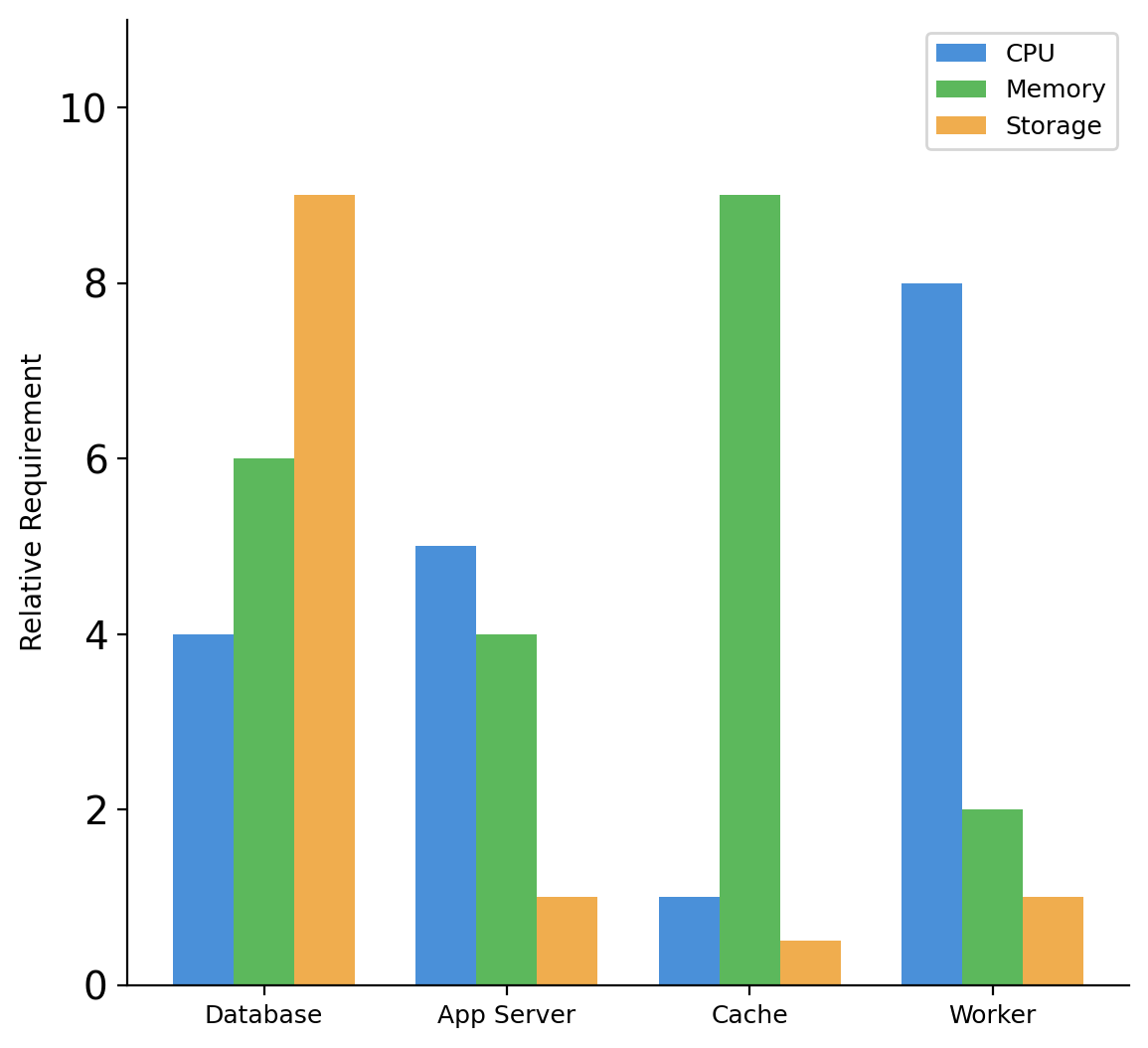
Resource Requirements Differ by Component Type

Database

High storage (data persists)

Moderate memory (buffer pool, caches)

Variable CPU (query execution)

Web/Application server

Low storage (stateless)

Moderate memory (request handling)

Variable CPU (business logic)

Cache

No persistent storage

High memory (that’s the point)

Low CPU (simple operations)

Background worker

Low storage

Low memory (between jobs)

High CPU (during processing)

Bundling components together means provisioning for the maximum of each resource type across all workloads.

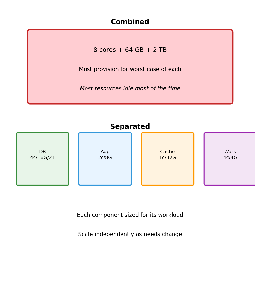
Separate Components Allow Independent Resource Allocation

Combined deployment on one machine:

8 CPU cores (for worker peaks)
64 GB memory (for cache)
2 TB storage (for database)
All resources allocated even when idle

Separate deployments:

Database: 4 cores, 16 GB, 2 TB storage
App server: 2 cores, 8 GB, minimal storage
Cache: 1 core, 32 GB, no storage
Worker: 4 cores, 4 GB, minimal storage

Total resources can be lower because each component gets what it needs, not what the most demanding component requires.

When one component needs more, scale that component. Others remain unchanged.

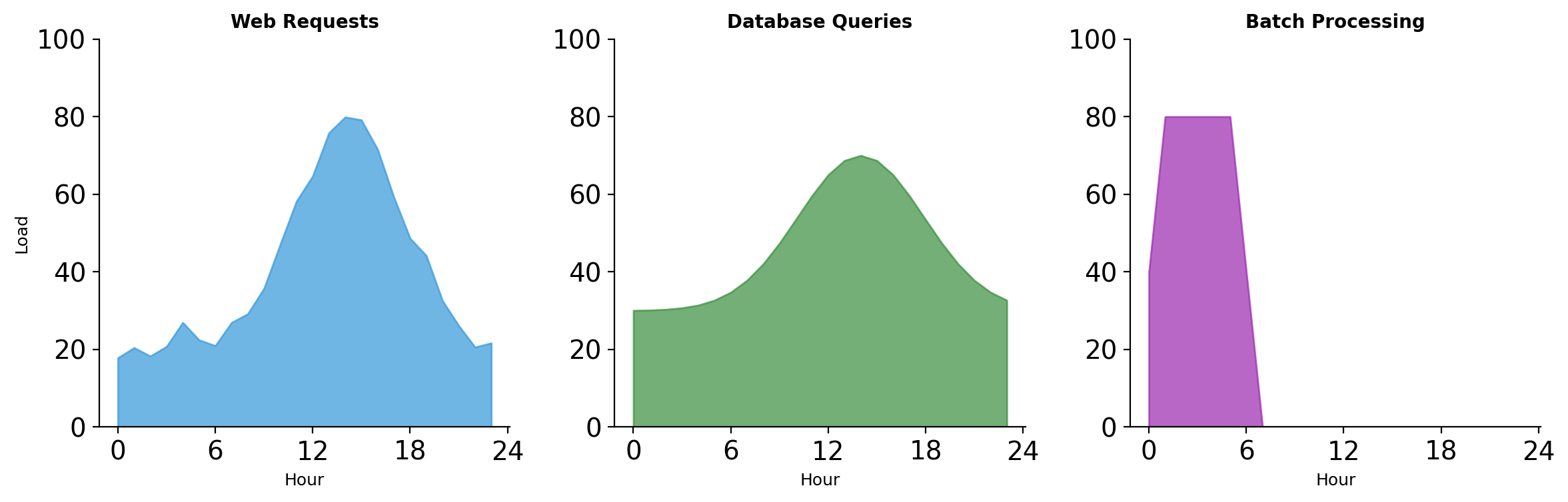
Traffic Patterns Vary by Component

Web traffic peaks during business hours. Batch jobs run overnight when web traffic is low.

Combined deployment: must handle peak web traffic + batch processing simultaneously (even though they naturally offset).

Separate deployment: web servers scale up during day, batch workers scale up at night. Total capacity can be lower because peaks don’t overlap.

Failure Containment Through Process Boundaries

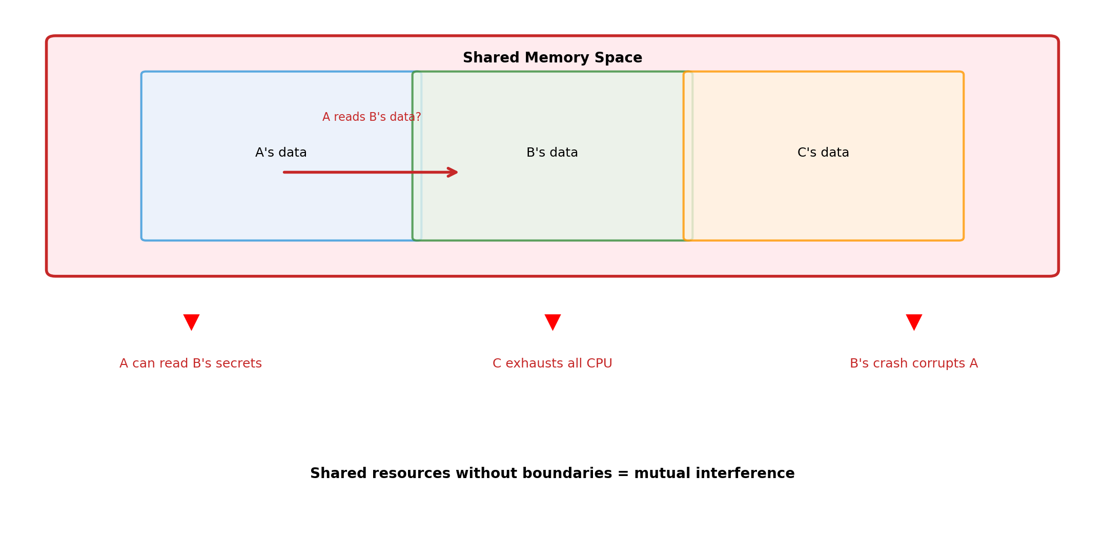
Process boundaries create failure domains. A crash in one process cannot corrupt memory in another.

Secrets Stay Within Their Boundaries

Component	Has Access To	Does Not Have
Web Server	TLS certificates	Database credentials
App Server	Database credentials	Payment API keys
Payment Service	Payment API keys	User session data
Background Worker	Job queue credentials	Direct user access

Compromise of one component limits exposure. Attacker who breaches the web server cannot read the database directly—must breach the app server separately.

Each boundary requires a separate exploit. Defense multiplies.

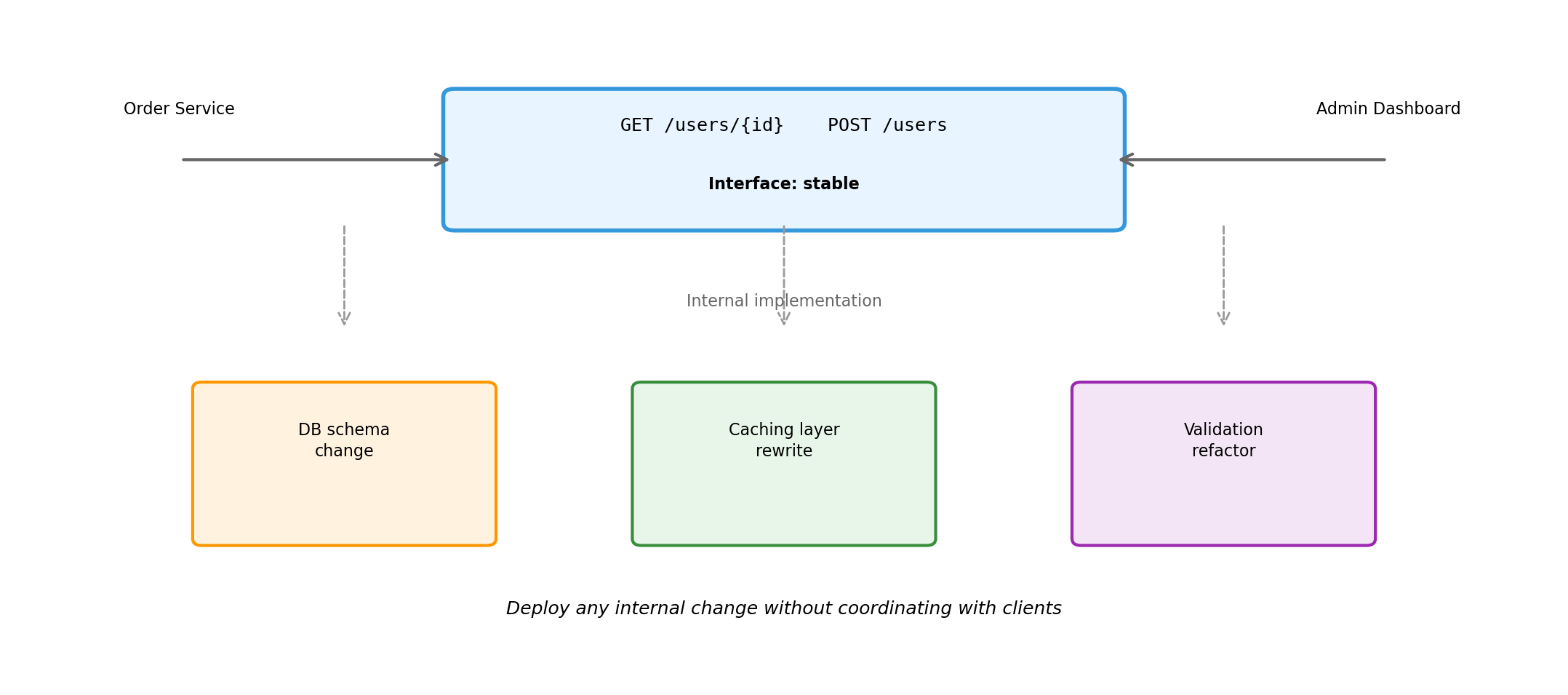
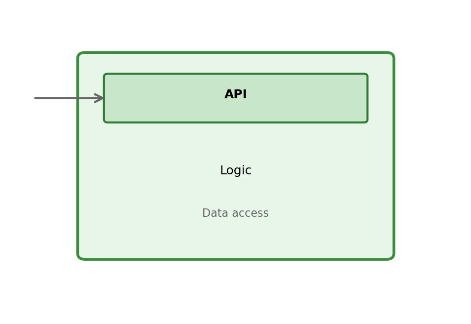
Interface Stability Enables Independent Deployment

External interface defines the contract. Internal changes—database migrations, caching strategies, validation logic—are invisible to clients.

Interfaces Enable Component Substitution

Scenario	Interface	Old Implementation	New Implementation	Client Change
Database migration	SQL protocol	MySQL	PostgreSQL	Connection string
Managed cache	Redis protocol	Self-hosted Redis	ElastiCache	Endpoint config
Search upgrade	Query API	Custom code	Elasticsearch	API adapter
Email provider	SMTP / HTTP API	Self-hosted	SendGrid	Credentials

Standard interfaces mean implementations are interchangeable. The component behind the interface can change—upgraded, replaced, outsourced—without rewriting clients.

Applications Compose Existing Capabilities

Writing 10,000 lines to compose millions of lines of specialized infrastructure.

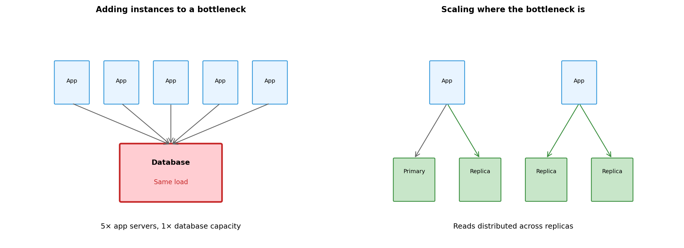
Distribution Enables Scaling (But Does Not Guarantee It)

Scaling requires decomposing along boundaries that allow independent scaling. Distribution makes decomposition possible. Architecture determines whether scaling works.

Distribution Requires Justification

Benefit	Cost
Specialized components	Explicit coordination
Independent resource allocation	Network uncertainty
Failure containment	Partial failure handling
Security boundaries	Operational complexity
Deployment independence	Interface management
Composition from existing systems	Distributed debugging

The benefits must outweigh the costs for the specific system being built. A system that doesn’t need failure containment, security boundaries, or independent scaling pays the coordination cost without receiving the benefit.

The Cloud Model

Infrastructure as Services Over a Network

Traditional model:

Buy servers, install in datacenter
Buy storage arrays, configure RAID
Buy network equipment, cable everything
Hire staff to maintain, monitor, replace

Cloud model:

Compute exists as a service you request
Storage exists as a service you request
Networking exists as a service you request
Provider operates the physical infrastructure

You don’t own resources. You consume them through APIs.

Cloud Providers Run Distributed Systems So You Can Run Yours

When you request a database, you’re calling a service. That service coordinates with storage services, networking services, monitoring services. Distributed systems all the way down.

Every Resource Is a Network Endpoint

Storage is not a local disk. It’s a service at a URL.

https://s3.us-east-1.amazonaws.com/my-bucket/my-file.csv

Database is not a local process. It’s a service at a hostname.

my-database.abc123.us-east-1.rds.amazonaws.com:5432

Your application component makes network requests to:

Other application components (your code)
Infrastructure services (provider’s code)

Same communication model. Same coordination challenges. Some endpoints you wrote, some you’re renting.

Requesting Resources: API Calls to Provider Services

Creating a storage bucket:

import boto3
s3 = boto3.client('s3')
s3.create_bucket(Bucket='my-application-data')

What happens:

Your code sends HTTPS request to S3 service
S3 service validates credentials, checks quotas
S3 service allocates storage, configures access
S3 service returns success (or error)
Bucket now exists as a network-accessible endpoint

You sent a message. A distributed system processed it. Resources appeared.

Storing Data: Messages to Storage Services

# Write
s3.put_object(
    Bucket='my-application-data',
    Key='users/12345.json',
    Body=json.dumps(user_data)
)

# Read
response = s3.get_object(
    Bucket='my-application-data',
    Key='users/12345.json'
)
user_data = json.loads(response['Body'].read())

Every read and write is a network request. The storage service handles:

Durability (replicating data across physical devices)
Availability (serving requests despite hardware failures)
Consistency (ensuring reads see recent writes)

The coordination problems exist. The provider solves them. You pay for the service.

The Provider Handles Certain Failures

Hardware disk fails:

Provider’s problem
Storage service has replicas
Your application doesn’t notice

Physical server overheats:

Provider’s problem
Workload migrates to other hardware
Your application may restart, but doesn’t manage the migration

Network switch fails in datacenter:

Provider’s problem
Redundant paths route around failure
Your application sees brief latency spike (maybe)

You Handle Other Failures

Storage service returns error:

Your problem
Retry? Fail gracefully? Alert?

Database connection times out:

Your problem
Is the database overloaded? Network partition? Configuration error?

Service in another region unreachable:

Your problem (mostly)
Provider guarantees region independence, not cross-region connectivity

The provider guarantees their components work. They don’t guarantee your application handles failures correctly.

Understanding the Boundary Matters

When something breaks, knowing which side of the boundary helps:

Provider side: check status page, wait, retry
Your side: check logs, fix code, redeploy

Configuration Replaces Construction

Describing what you want:

# "I want a PostgreSQL database"
database:
  engine: postgres
  version: "14"
  storage: 100GB
  backup: daily

Provider figures out:

Which physical hardware to use
How to configure replication
Where to store backups
How to handle failover

You declare intent. Provider handles implementation.

Infrastructure Described in Code

# docker-compose.yml
services:
  web:
    image: nginx
    ports:
      - "80:80"

  api:
    build: ./api
    environment:
      DATABASE_URL: postgres://db:5432/app

  db:
    image: postgres:14
    volumes:
      - db-data:/var/lib/postgresql/data

Three services. Their relationships. Their configuration.

Run docker-compose up. Infrastructure exists.

Change the file. Run again. Infrastructure updates.

Delete the file. Run down. Infrastructure gone.

Resources Can Scale Because They’re Services

Fixed hardware:

10 servers purchased
Traffic exceeds capacity
Order more servers (weeks)
Install, configure (days)
Traffic already gone

Resources as services:

Request 10 compute units
Traffic exceeds capacity
Request 20 compute units (seconds)
Traffic subsides
Release 15 compute units (seconds)

Scaling is an API call, not a procurement process.

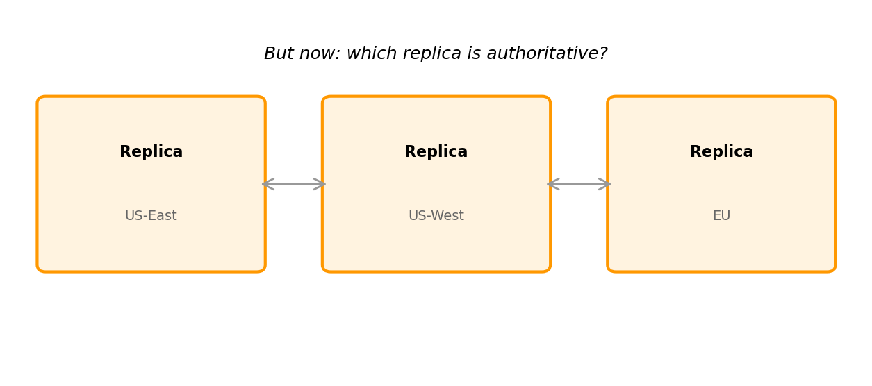
Geographic Presence Through Configuration

Provider operates datacenters in multiple regions:

Region	Location	Use Case
us-east-1	N. Virginia	Primary US
eu-west-1	Ireland	European users, GDPR
ap-northeast-1	Tokyo	Asian users

Deploy to a region by specifying it in configuration:

s3 = boto3.client('s3', region_name='eu-west-1')

Physical presence in Frankfurt, Tokyo, São Paulo—without owning datacenters there.

What Cloud Changes

Traditional	Cloud
Own hardware	Rent services
Build infrastructure	Configure infrastructure
Fixed capacity	Elastic capacity
Capital expense	Operational expense
Provision in weeks	Provision in seconds
Limited geography	Global presence

What doesn’t change:

Coordination challenges between components
Network communication model
Need to handle failures
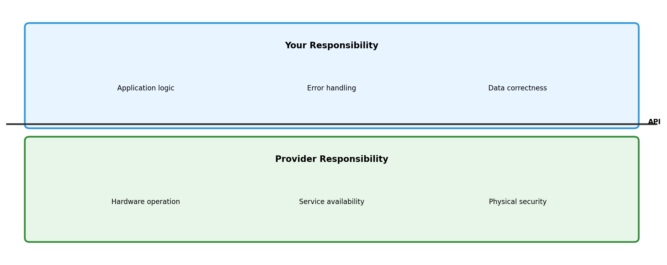
Application design responsibility

Cloud shifts where the infrastructure comes from. It doesn’t eliminate the distributed systems problems—it gives you building blocks to construct solutions.

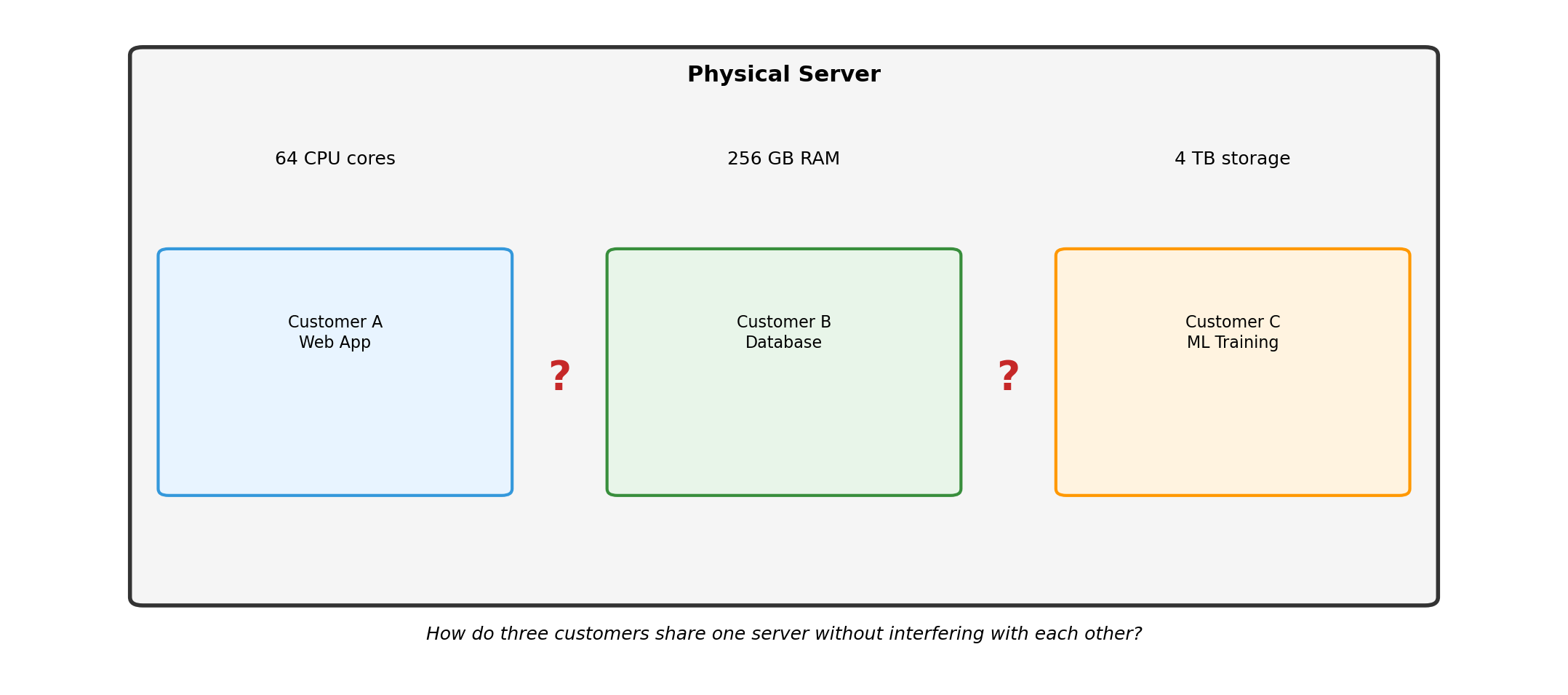
Isolation and Virtualization

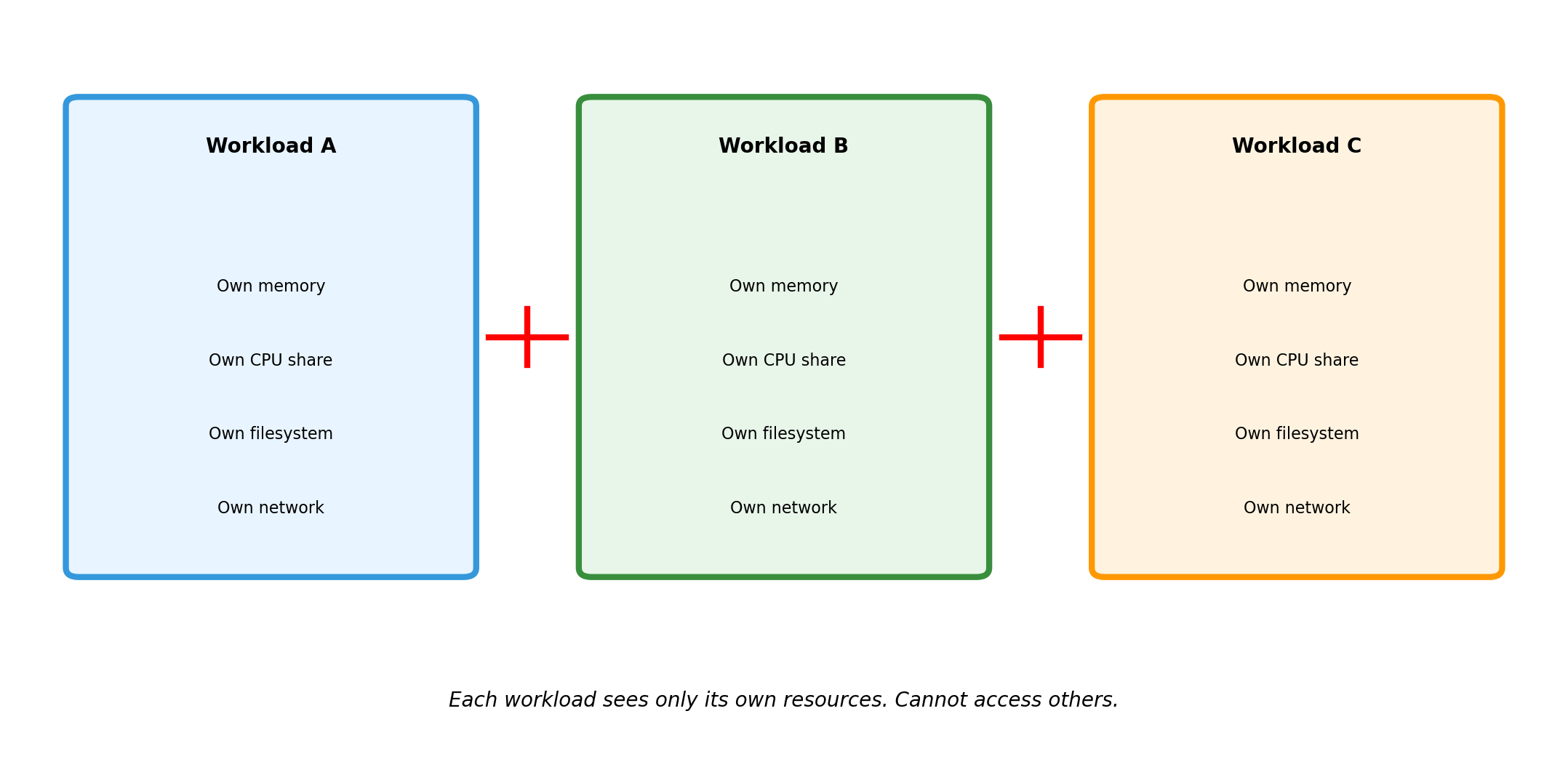
Multiple Workloads, Shared Hardware

Without Isolation: Interference

Isolation Creates Boundaries

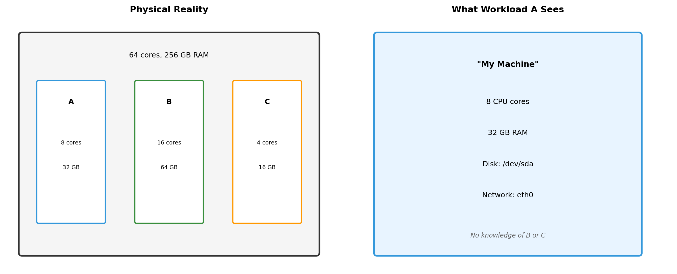
What Each Isolated Environment Sees

Workload A cannot detect that B and C exist. It sees a complete machine with its allocated resources. The isolation is invisible from inside.

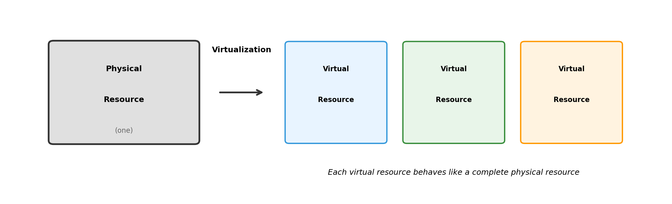
Virtualization: Making One Thing Look Like Another

Virtualization creates an abstraction that behaves like the real thing.

Software interacting with a virtual resource doesn’t know it’s virtual. The abstraction is complete.

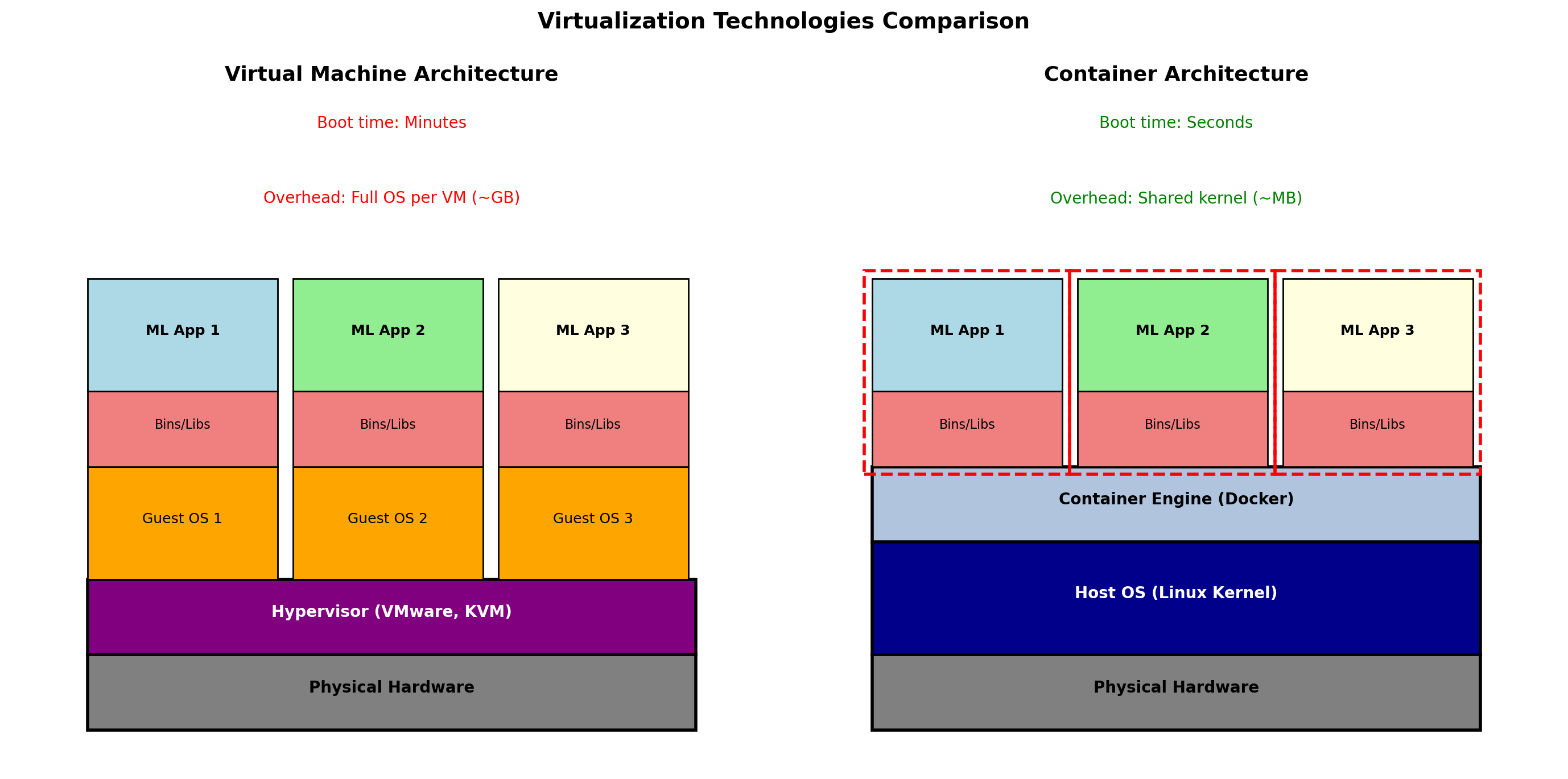
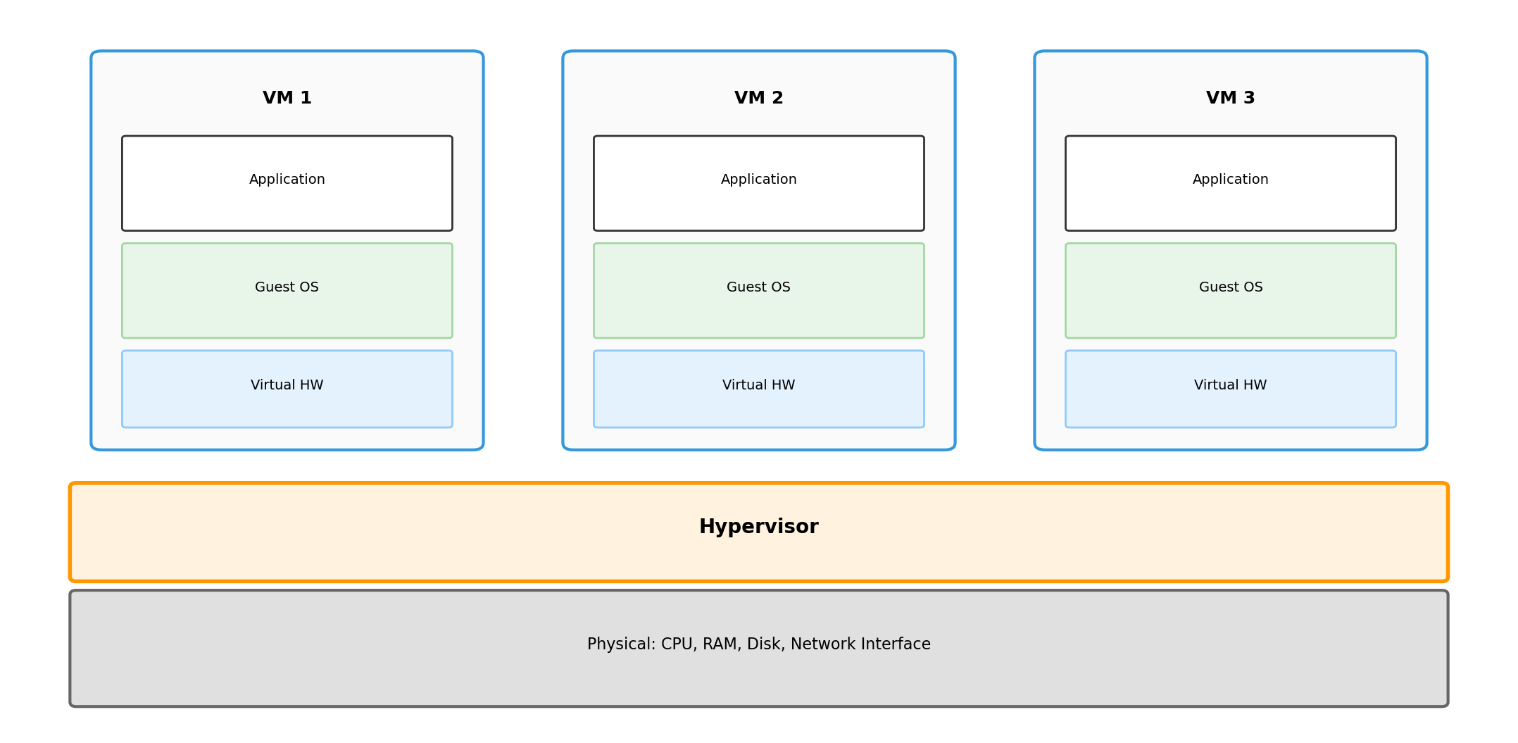
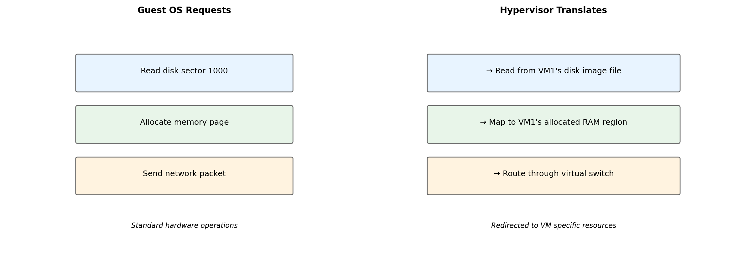
Virtual Machines: Virtualize Hardware

A hypervisor sits between physical hardware and guest operating systems.

Each VM gets virtualized CPU, RAM, disk, network. Guest OS runs unmodified—it believes it has real hardware.

The Guest OS Cannot Tell the Difference

The guest OS issues normal hardware instructions. The hypervisor intercepts and redirects them to the VM’s allocated resources. Isolation enforced transparently.

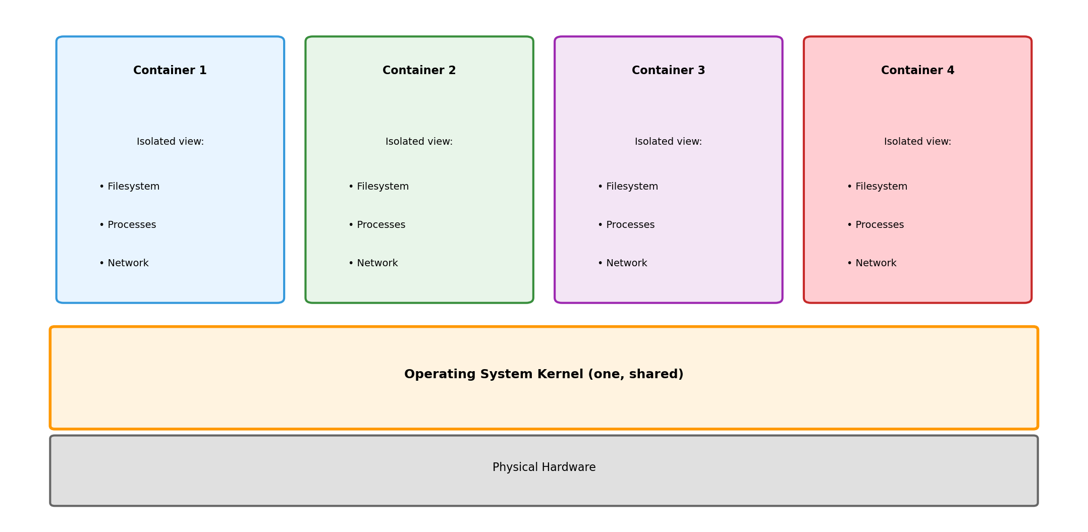
Containers: Virtualize the Operating System

Instead of virtualizing hardware, containers virtualize the OS environment.

All containers share the same kernel. Each container sees an isolated view of the filesystem, process list, network.

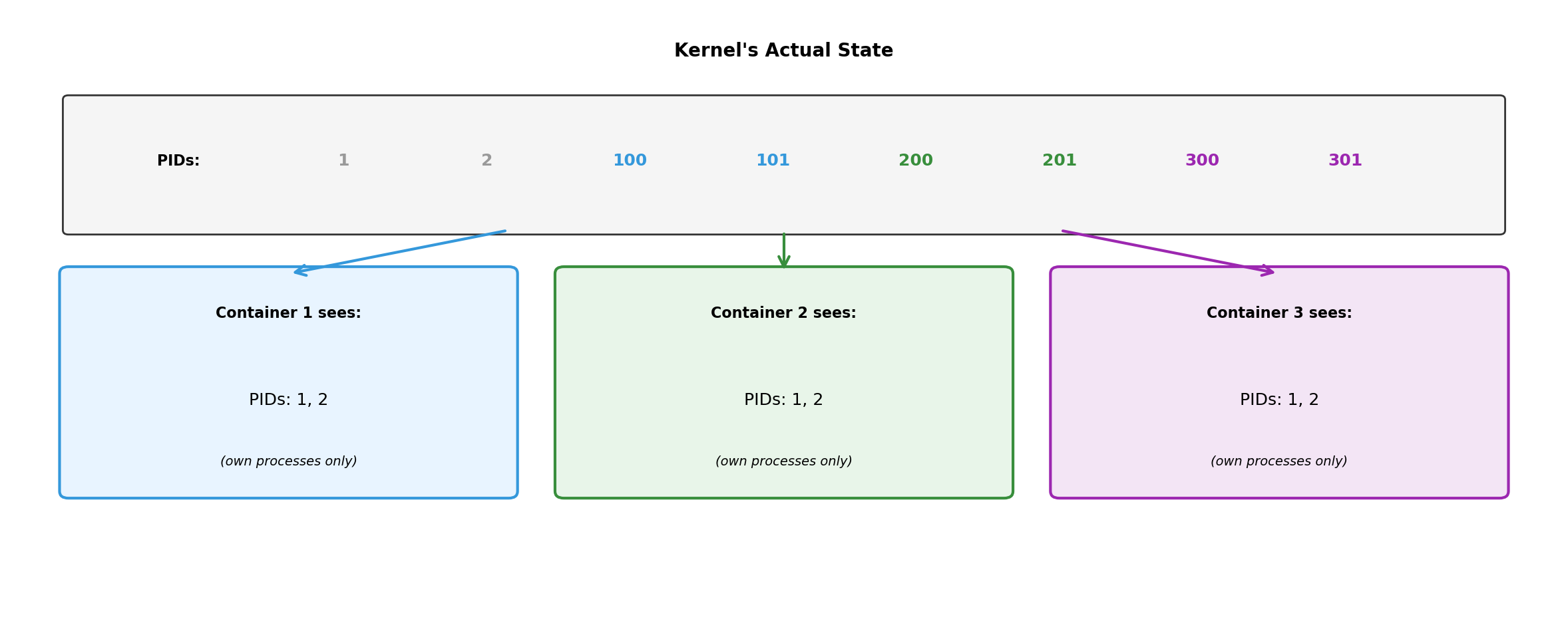
Same Kernel, Different Views

Kernel tracks all processes. Each container’s view is filtered—it sees only its own processes, starting from PID 1.

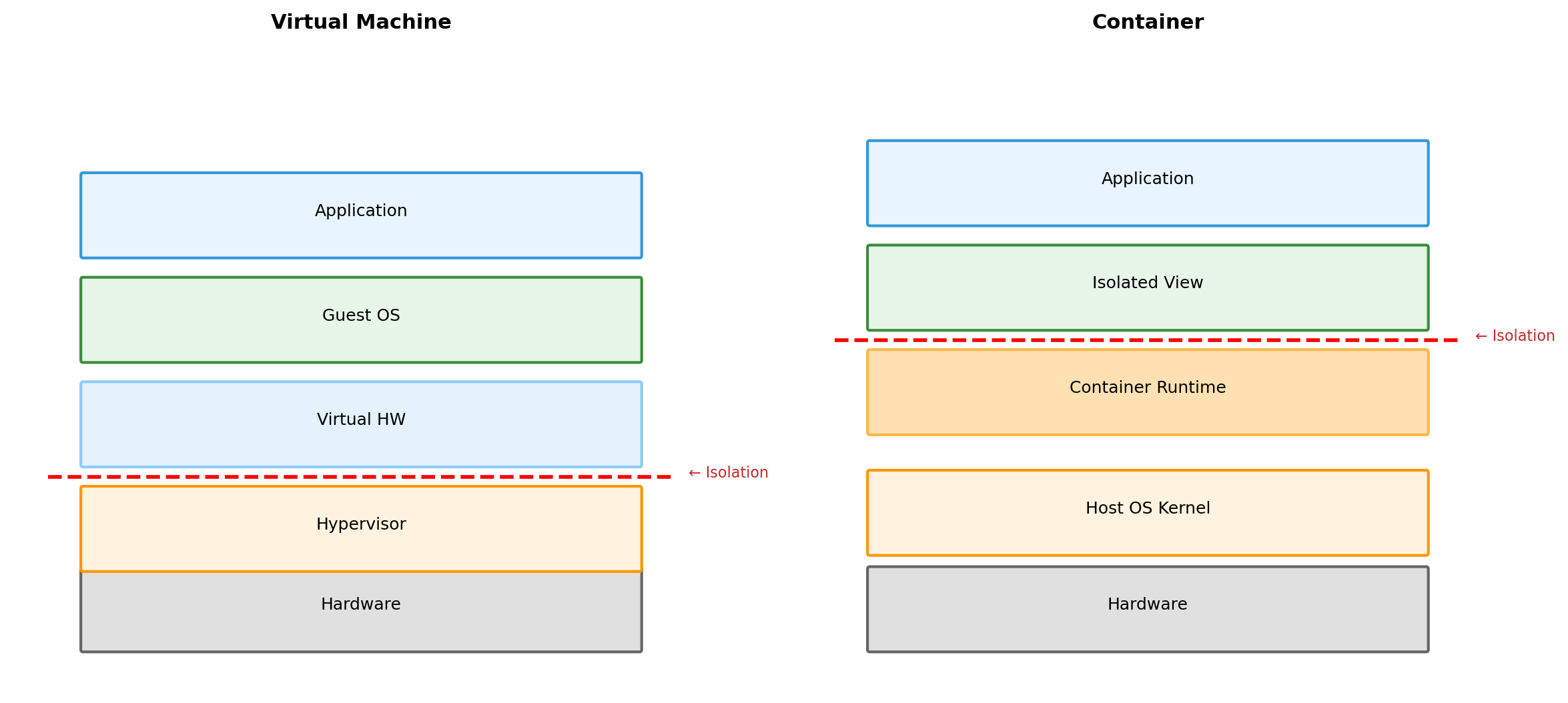
VMs vs Containers: Different Layers of Virtualization

VM isolation at hardware boundary (hypervisor). Container isolation at OS boundary (kernel features).

Containers for This Course

Containers are the practical deployment unit:

Lightweight: Start in milliseconds, minimal overhead
Portable: Same container runs on laptop and cloud
Composable: Multiple containers form distributed system

Each component of a distributed application runs in its own container. Containers communicate over the network—same model as Section 1.

Later lectures cover container mechanics in depth. For now: containers provide isolation boundaries for application components.

From Isolation to Distributed Systems

Communication

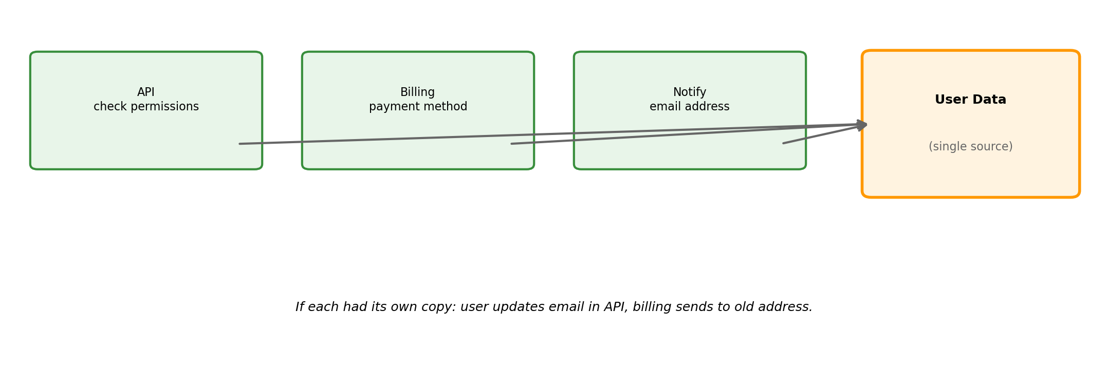
Isolated Components Must Exchange Information

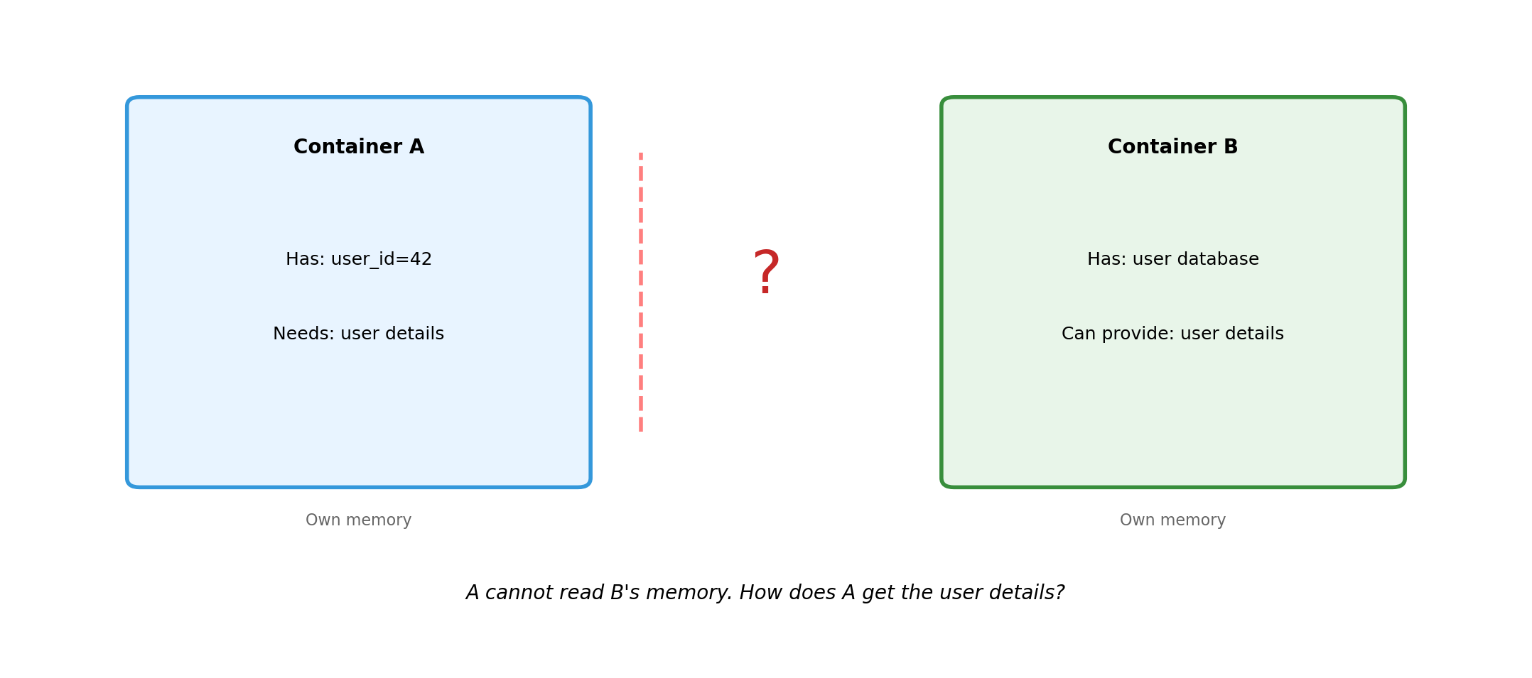
Message Passing Replaces Shared Memory

Coordination requires explicit communication. Every piece of shared information must be copied across the network.

All Coordination Through Messages

In a distributed system, components coordinate exclusively through messages:

No shared variables - cannot read another component’s memory
No shared locks - mutex doesn’t work across machines
No function calls - cannot invoke code in another process

Every coordination mechanism reduces to: send a message, receive a response.

This is fundamentally different from single-process coordination where threads can share memory, signals, and synchronization primitives.

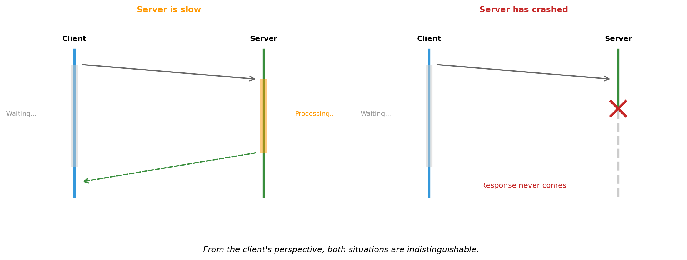
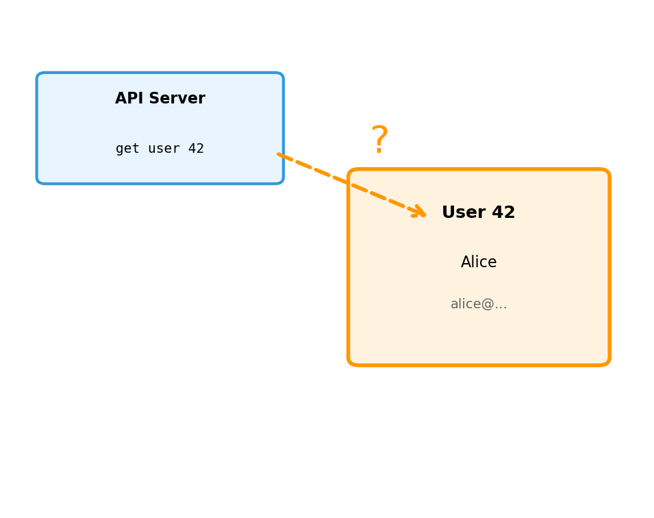
Network Behavior Is Uncertain

Slow and Failed Look Identical

Timeouts are guesses. A timeout expiring means “no response yet” - not “server is dead.”

Protocols Define Message Structure

A protocol establishes rules both parties agree to follow:

What protocols specify:

Message format and encoding
Valid operations and their meanings
Expected response types
Error signaling conventions

Why protocols matter:

Sender and receiver must parse messages the same way
Operations must have consistent semantics
Errors must be recognizable as errors
Without agreement, communication fails

Protocols are contracts. HTTP, TCP, DNS, SMTP - each defines a specific contract for a specific purpose.

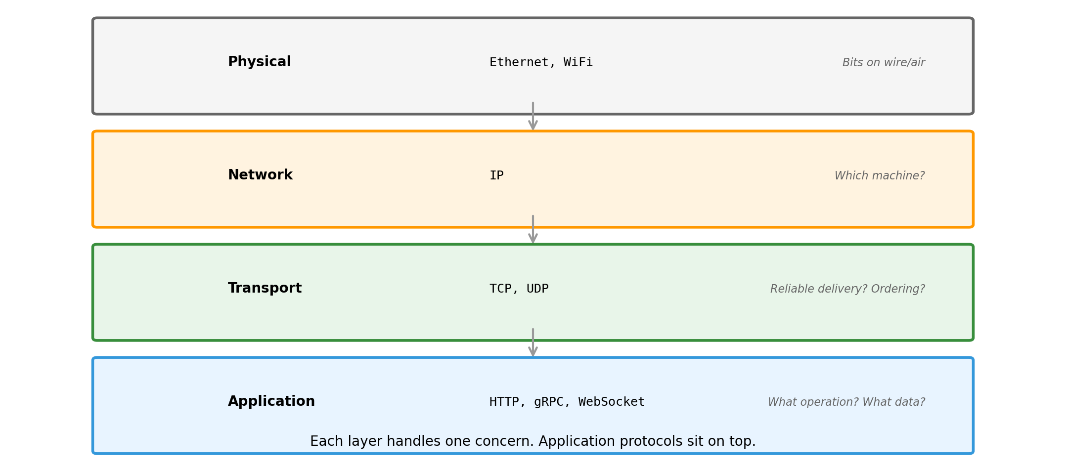
Protocols at Different Layers

We work primarily at the application layer. TCP handles reliable delivery underneath.

HTTP: Common Application Protocol

HTTP (Hypertext Transfer Protocol) is widely used for service communication:

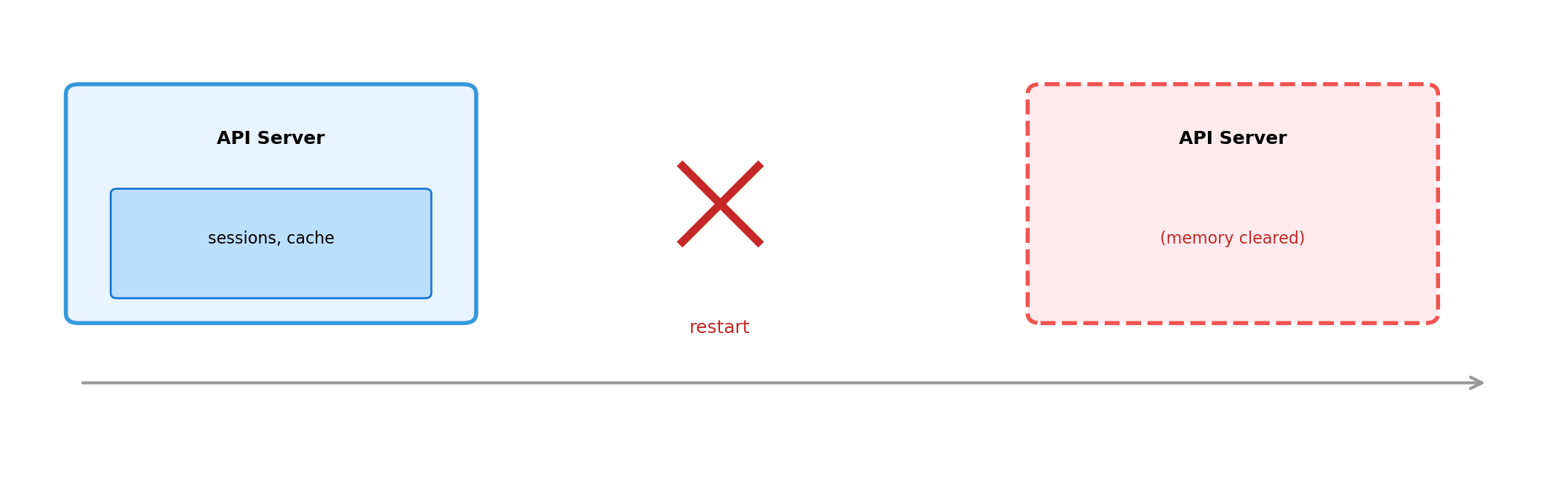
Request-response model - client sends request, server sends response
Stateless - each request is independent; server keeps no memory of client between requests
Text-based - human-readable format (helpful for debugging)
Extensible - headers allow adding metadata without changing core protocol

Originally designed for web browsers. Now the default for APIs, cloud services, and service-to-service communication.

Details of HTTP syntax and semantics come in later lectures when we build APIs.

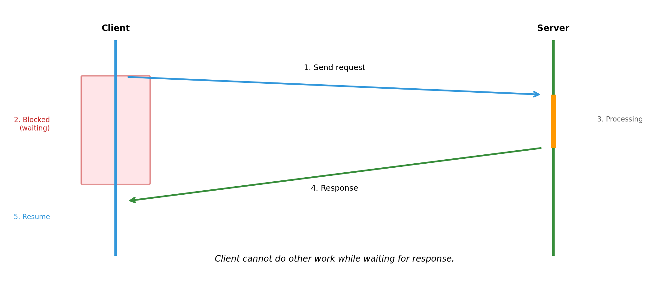
Synchronous Communication Blocks the Caller

Simple model: send, wait, receive. But waiting time is wasted if client could do other work.

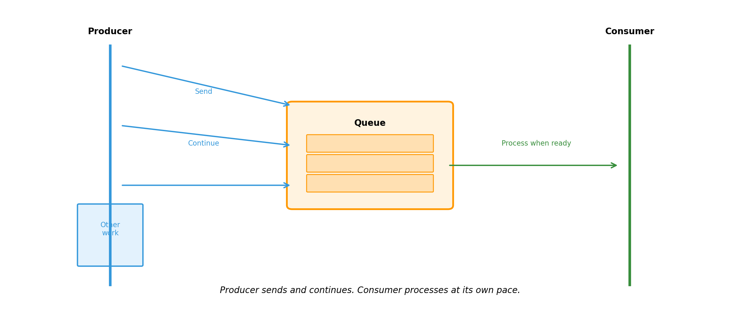
Asynchronous Communication Decouples Sender and Receiver

Synchronous vs. Asynchronous: Trade-offs

Synchronous

Immediate feedback
Simple error handling (error returns with response)
Easy to reason about
Caller blocked until completion
Tight coupling in time

Asynchronous

No blocking; better resource utilization
Producer and consumer scale independently
Handles burst traffic via buffering
Complex error handling (how do errors get back?)
Messages may sit in queue indefinitely

Neither is universally better. Choice depends on:

How quickly does caller need the result?
Can the operation tolerate delay?
What happens if the receiver is temporarily unavailable?

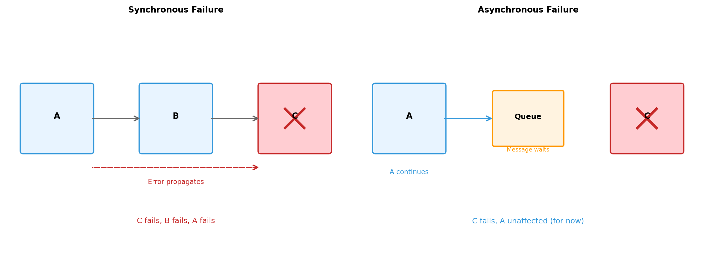
Failure Modes Differ by Communication Style

Asynchronous communication isolates failures temporally. But errors still need handling eventually.

Communication Shapes System Design

How components communicate affects everything:

Latency budget - synchronous chains multiply delays
Failure isolation - async provides buffering against downstream problems
Consistency - synchronous makes coordination easier; async makes it harder
Coupling - synchronous couples components in time; async decouples them

Every inter-component boundary is a communication decision. These decisions accumulate into system-wide characteristics.

Later lectures address these trade-offs in depth: API design, async patterns, failure handling strategies.

State and Persistence

Messages Reference Data That Lives Somewhere

get user 42 expects user 42 to exist:

Name, email, creation date, preferences
Existed before this request
Will exist after this request
Survives if the API server restarts

This is state - persistent information that requests read and modify.

In a distributed system, the component making a request may be on a different machine than where the data lives.

Memory State Dies with the Process

Deployments, crashes, scaling events, orchestrator decisions - all clear memory.

For ephemeral data (request context, short caches), this is fine. For user data, orders, anything important - memory-only is unacceptable.

Shared State Requires a Shared Location

When multiple components need the same data, it must live somewhere all can reach:

State Requirements Lead to External Storage

Durability

Must survive component restarts

→ Cannot live only in memory

Accessibility

Must be reachable by multiple components

→ Must be network-accessible

Components read/write to external store. Components can restart without losing data.

Databases as Coordination Points

A database centralizes state management for distributed components:

Role	What It Provides
Location	Single endpoint all services reach
Durability	Data survives component failures
Concurrency	Handles simultaneous readers/writers
Query	Find by ID, search, filter, aggregate

Without this, each service would implement its own storage, replication, concurrency control, and query logic.

Concurrent Writers Can Conflict

Both read 100, compute independently, write back. B’s write overwrites A’s change.

State Coordination Echoes Threading Coordination

Threads (shared memory)

Race conditions on variables
Locks, mutexes
Deadlock, livelock risks
Hard despite same machine

Distributed state (shared database)

Race conditions on records
Transactions, isolation levels
Distributed deadlock possible
Network adds uncertainty

Same fundamental problem: independent agents accessing shared mutable state.

Databases provide coordination mechanisms (transactions, locking, isolation). Using them correctly requires understanding why the problem exists.

Different State, Different Access Patterns

One application may have fundamentally different kinds of data:

A storage system optimized for one pattern may perform poorly for another.

Storage Systems Optimize for Specific Patterns

Relational (PostgreSQL, MySQL)

Structured schemas, SQL
ACID transactions
Flexible queries
General purpose

Key-Value (Redis, DynamoDB)

Get/put by key
Very fast lookups
Limited query flexibility
Sessions, caches

Document (MongoDB)

Flexible schemas
Nested structures
Query within documents

Specialized

Time-series: append-optimized, range queries
Graph: relationship traversal
Vector: similarity search, embeddings
Column: analytics workloads

Mismatch Costs

Relational for everything

Embeddings similarity search: works, but 100x slower than vector DB

Time-series at scale: complex partitioning, custom indexing

Sessions: paying for ACID guarantees you don’t need

Specialized for everything

Key-value for complex queries: joins in application code

Multiple systems: operational overhead, data sync challenges

Wrong tool for simple cases: complexity without benefit

The question isn’t “which database is best” but “what does this specific state require.”

State Itself Can Be Distributed

Single database → potential bottleneck, single point of failure.

Replication addresses this:

Durability: copies survive failures
Read scaling: distribute load
Geography: data closer to users

Replication Forces Consistency Choices

Strong consistency

All replicas agree before acknowledging writes

Readers always see latest value
Writes slower
May reject operations during partitions

Eventual consistency

Writes acknowledge immediately; replicas sync later

Faster writes, higher availability
Readers may see stale data
Application handles temporary inconsistency

Banking transaction: strong consistency required.

Social media like count: eventual consistency acceptable.

Requirements determine the appropriate choice.

State Decisions Cascade

Choice	Consequences
Where state lives	Latency, failure domains, operational responsibility
Storage system	Query capabilities, throughput limits, consistency model
Replication strategy	Durability guarantees, read scaling, consistency trade-offs
Consistency level	Application correctness constraints, availability during failures

No configuration optimizes all dimensions. State architecture is choosing which trade-offs to accept.

Services and Composition

Distributed Applications Are Built from Services

A service is an independent process that:

Runs as its own process (or container)
Exposes a network interface (API)
Encapsulates specific functionality
Manages its own data (or accesses shared stores)
Can be deployed independently

Not a library you link against - a running process you communicate with over the network.

Services Enable Independent Operation

Each service can be:

Dimension	Independence Means
Developed	Different team, different pace, different language
Deployed	Update one service without redeploying others
Scaled	Add instances of high-load services only
Failed	One service crashing doesn’t necessarily crash others

This independence comes from the network boundary - services interact through defined interfaces, not shared memory or direct function calls.

A Typical Application Structure

APIs Define Service Boundaries

An API (Application Programming Interface) specifies:

What’s exposed

Available operations
Required inputs
Response formats
Error conditions

This is the contract clients depend on.

What’s hidden

Internal data structures
Implementation language
Database schema
Performance optimizations

Implementation can change without breaking clients.

Interface Stability Enables Independence

If interface is stable:

Service team refactors internals freely
Database schema can evolve
Performance optimizations don’t break callers
New features added without coordination

Services evolve independently.

If interface changes:

All callers must update
Coordination required across teams
Deployment coupling returns
Version management complexity

Breaking changes propagate.

API design and versioning are significant engineering challenges. A poorly designed API creates coupling that undermines service independence.

Services Call Other Services

A user request often traverses multiple services:

Composition Has Costs

Each service boundary adds:

Cost	Impact
Latency	Network round-trip per hop (typically 1-50ms each)
Failure probability	Each service is an additional failure point
Complexity	Debugging spans multiple processes, logs, traces
Operational overhead	More services = more to deploy, monitor, maintain

A request traversing 5 services with 99% availability each: 0.99^5 = 95% success rate.

Service boundaries are not free. They exist where independence benefits outweigh coordination costs.

Downstream Failures Affect Upstream Callers

Slow Services May Be Worse Than Failed Services

Service fails fast

Caller gets error immediately
Can return error to user
Can try fallback
Resources freed quickly

Unpleasant but bounded.

Service responds slowly

Caller waits (blocking thread/connection)
Timeout eventually fires
Resources held during wait
Slow responses back up, causing cascading slowness

Can exhaust caller’s resources.

A service responding in 30 seconds instead of 30ms can cause more damage than one that fails immediately.

Timeouts Are Essential but Imperfect

Every service call needs a timeout - but choosing timeout values is hard:

Timeout too short

Gives up on requests that would succeed
Increases error rate unnecessarily
May trigger retries that add load

Timeout too long

Resources held waiting
Slow responses back up
User already gave up, but system still working

Timeout = how long are you willing to wait before assuming failure? There’s no universally correct answer.

Retries Can Help or Hurt

When a request fails, should the caller retry?

Retries help when:

Failure was transient (network blip, temporary overload)
Request is idempotent (safe to repeat)
Downstream service has recovered

Retries hurt when:

Downstream is genuinely overloaded (retries add load)
Many callers retry simultaneously (thundering herd)
Request is not idempotent (duplicate side effects)

Retry strategies (exponential backoff, jitter, limits) are necessary but add complexity.

Circuit Breakers Prevent Cascade Failures

When a downstream service is failing, continuing to call it:

Wastes resources on requests that will fail
Adds load to an already struggling service
Slows down the caller waiting for timeouts

Circuit breaker: fail fast when downstream is unhealthy, periodically test for recovery.

Designing for Partial Failure

In a distributed system, something is always failing somewhere. Services must handle:

Downstream services being unavailable
Slow responses from dependencies
Network partitions between components
Partial results when some calls succeed and others fail

Graceful degradation: return partial results, use cached data, disable features - rather than complete failure.

This is a design concern from the start, not something to add later.

Services Are the Structure of Distributed Applications

The concepts from earlier sections manifest through services:

Concept	How It Appears
Isolation (Section 4)	Each service in its own container
Communication (Section 5)	Services interact via APIs over network
State (Section 6)	Services manage or share state through databases
Coordination (Section 1)	Service interactions require coordination patterns

Building distributed applications = designing services, their APIs, their interactions, and their failure modes.

EE 547: Synthesis

ML Training at Scale

Training a large model on a substantial dataset creates specific infrastructure requirements:

Data challenges

Dataset is 500GB - doesn’t fit in memory
Need to feed batches to GPU continuously
Multiple experiments use same dataset
Preprocessing should not block training

Compute challenges

Training takes hours or days
GPU time is expensive and limited
Failures happen - can’t restart from zero
Want to run multiple experiments

A single Python script on a laptop doesn’t scale to this. What infrastructure makes it tractable?

Data Must Be Accessible and Streamable

Object storage holds the dataset:

Network-accessible from any compute node
Durable - data survives node failures
Can store TBs economically

Data pipeline streams to training:

Fetches batches on demand
Preprocesses (augmentation, normalization)
Keeps GPU fed without loading full dataset

Training code sees an iterator of batches. Infrastructure handles the rest.

Long-Running Training Needs Fault Tolerance

A training run takes 8 hours. At hour 6, the node crashes. Without preparation: start over, lose 6 hours of GPU time.

Checkpointing solves this:

Save model weights periodically (every epoch, every N steps)
Save optimizer state, learning rate schedule
Write to durable storage (not local disk)
On restart: load latest checkpoint, continue

Checkpoints also enable:

Stopping and resuming intentionally
Branching experiments from a saved state
Recovering from preemption (spot instances)

Experiments Need Tracking and Comparison

Running many experiments creates a management problem:

Which hyperparameters produced which results?
How do loss curves compare across runs?
What code version was used for the best model?
Which checkpoint should go to production?

Experiment tracking captures:

What	Why
Hyperparameters	Reproduce the run
Metrics over time	Compare learning dynamics
Code version / git hash	Know exactly what ran
Final model location	Find the artifact

This is a service that training jobs write to - separate from the training code itself.

GPU Resources Need Scheduling

GPUs are expensive and limited. Multiple users/experiments compete for them.

Without orchestration:

Manual checking: “is a GPU free?”
Jobs sitting idle waiting for resources
No queuing - first-come first-served chaos
No preemption for priority jobs

With orchestration:

Submit job with resource requirements
Scheduler assigns to available GPU
Queue manages waiting jobs
Can preempt low-priority for high-priority

ML Training: Full Picture

Each component addresses a specific requirement. Data flows left-to-right; state persists in storage systems; orchestrator coordinates the whole.

Real-Time Transit Tracking

Different problem, similar structural patterns. A transit agency publishes vehicle positions. Build an application that:

Must handle:

Positions update every 15 seconds per vehicle
Hundreds of vehicles across the network
Users want current positions on a map
Users want alerts when their bus is delayed

Complications:

External API - we don’t control format or reliability
Delay detection requires computation (compare to schedule)
Web users expect fast responses
Notifications are asynchronous

Ingesting External Data

The transit API provides raw data, but:

Their format may be awkward (XML, custom schema)
Their uptime isn’t guaranteed
Polling rate limited - can’t request on every user query

Ingestion service handles this boundary:

Polls external API on schedule
Normalizes data to internal format
Handles external API failures gracefully
Publishes to internal queue for processing

Internal services never touch external API directly. Ingestion isolates that dependency.

Queue Decouples Ingestion from Processing

Positions arrive in bursts (all vehicles update near-simultaneously). Processing (delay detection) takes variable time.

Message queue between them:

Ingestion publishes events at arrival rate
Queue buffers bursts
Processors consume at their own pace
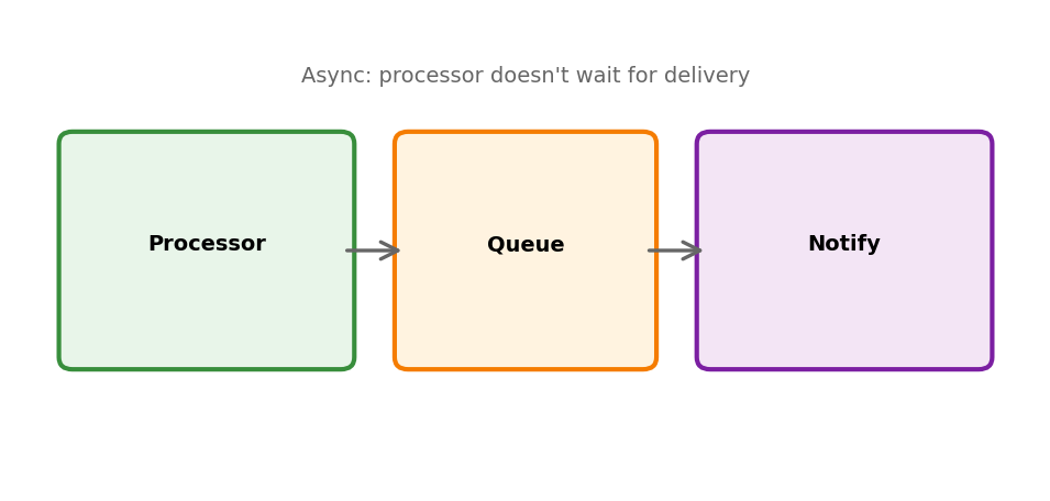
If processor is slow, queue grows (doesn’t block ingestion)
Can add more processors to increase throughput

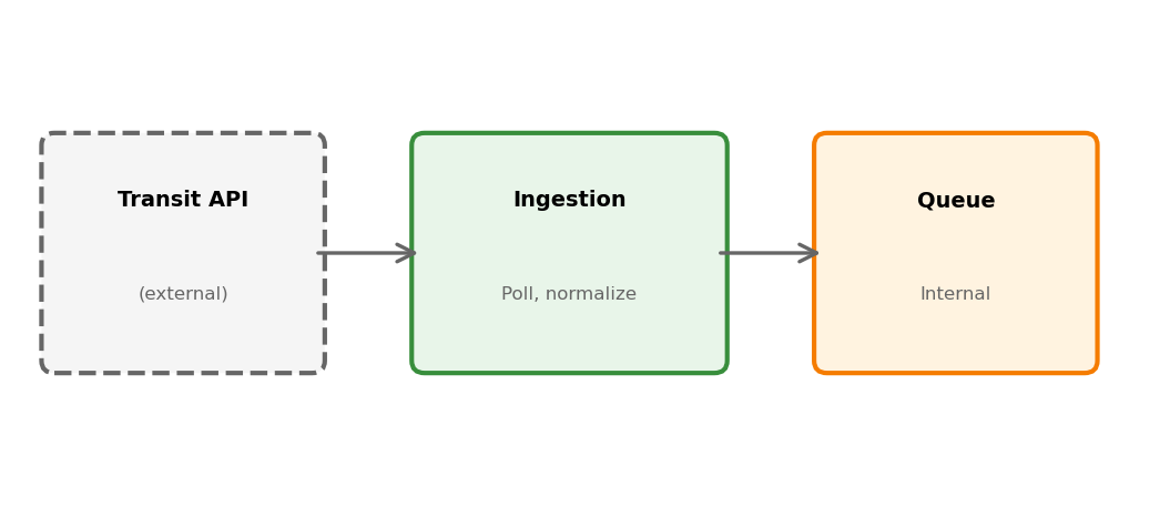
This is async communication from Section 5:

Producer continues without waiting
Consumer processes independently
Temporal decoupling between components

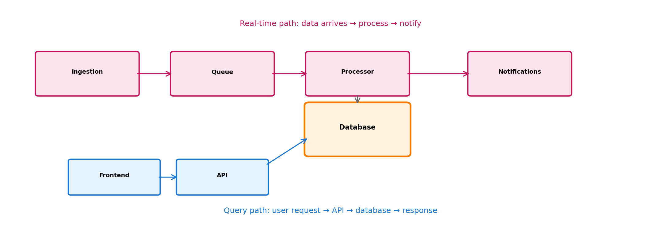
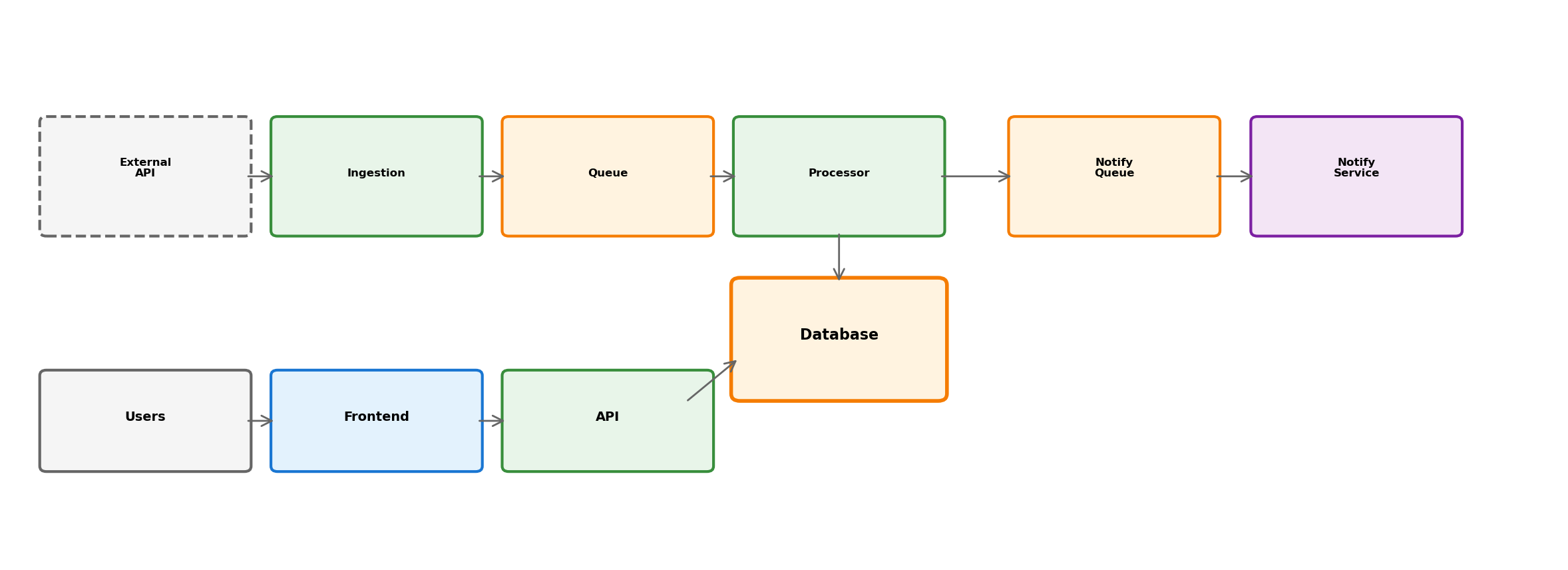
Two Data Paths: Real-Time and Query

Real-time: events flow through queue, processor detects delays, sends notifications.

Query: user requests current positions, API queries database, returns response.

Different patterns for different access types. Database is the meeting point.

Notifications Are Asynchronous

When processor detects a delay, it doesn’t send email directly. Instead:

Processor publishes “delay detected” event
Notification service consumes these events
Handles delivery (email, SMS, push)
Manages user preferences, rate limiting

Why separate?

Delivery is slow (network calls to external providers)
Don’t want delay in processing pipeline
Notification logic is complex (preferences, templates, retries)
Can fail independently without affecting detection

Transit App: Full Picture

External data enters through controlled boundary. Real-time and query paths serve different needs. Async processing prevents blocking. Components are independently deployable.

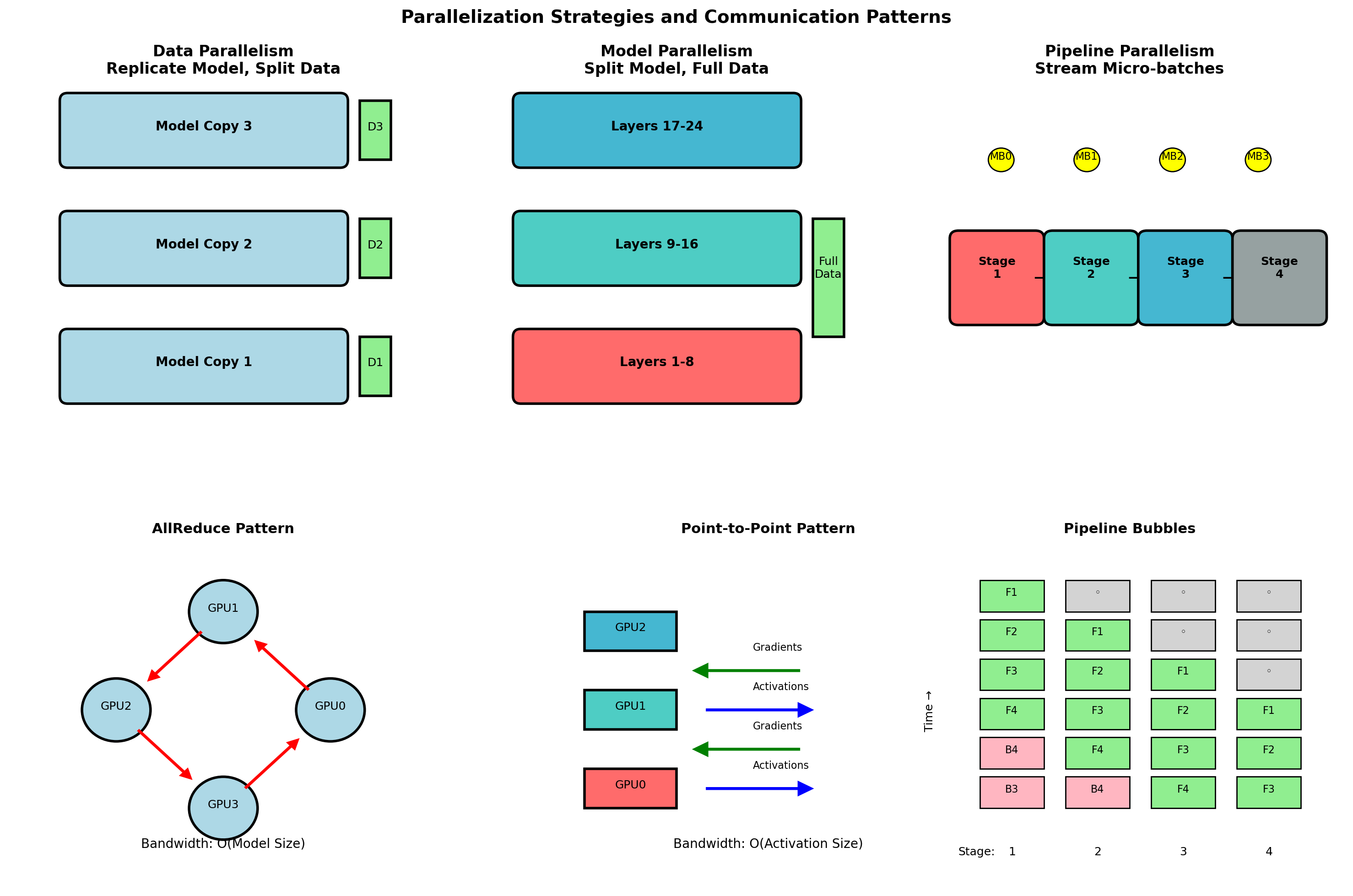
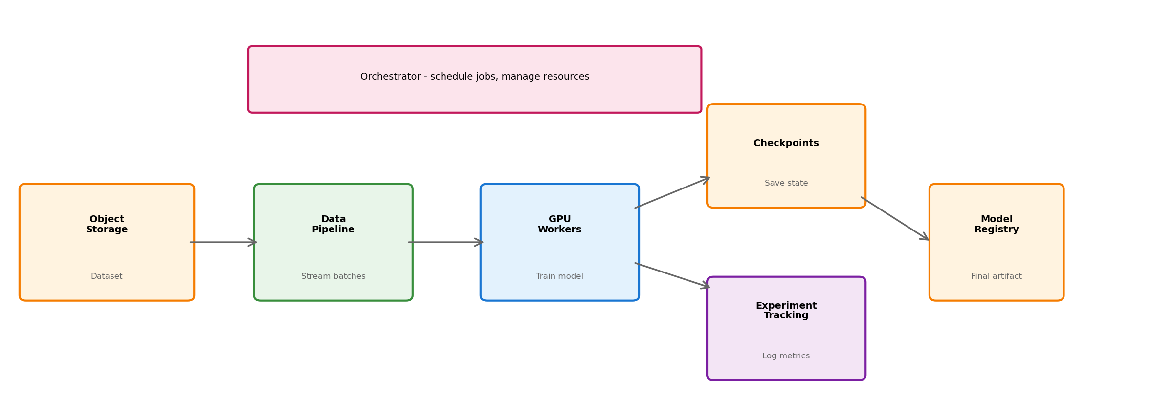
Patterns That Appear in Both

Pattern	ML Training	Transit App
External boundary	Object storage holds dataset	Ingestion service wraps external API
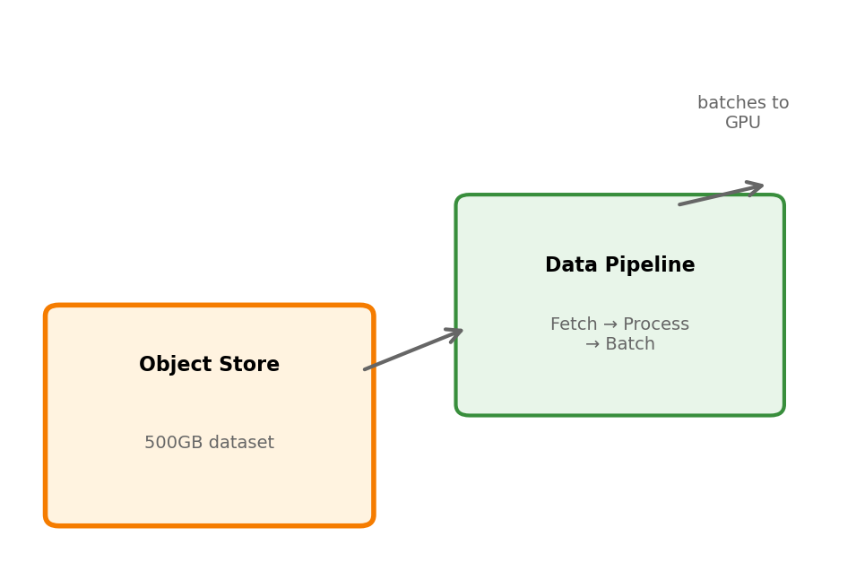
Async processing	Data pipeline feeds GPU workers	Queue between ingestion and processor
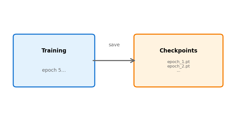
Durable state	Checkpoints, experiment logs	Database for positions and history
Separation of concerns	Training vs tracking vs scheduling	Ingestion vs processing vs notification
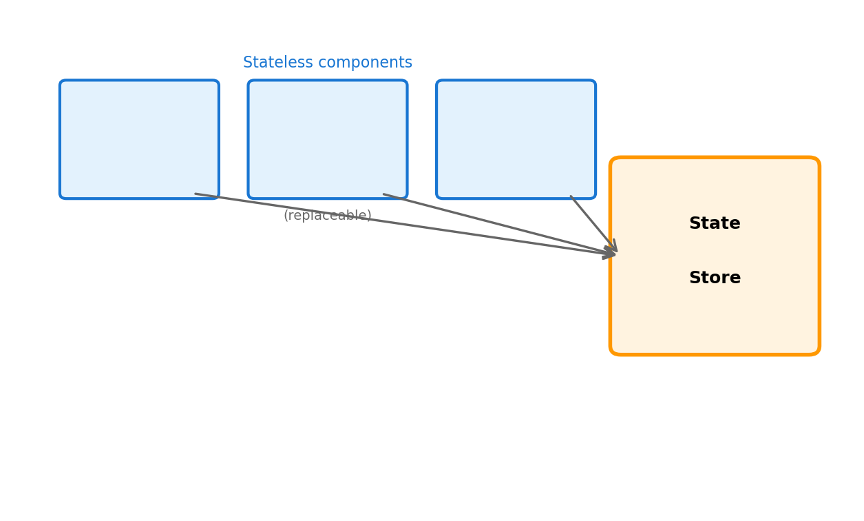
Stateless compute	Workers can restart, reschedule	Services can scale, restart

Different domains, same structural principles. The concepts from earlier sections appear as concrete components.