Containers and Orchestration
EE 547 - Unit 2
Each Process Needs Resources to Run
A process consumes physical resources:
CPU — executes instructions, handles requests
The database process needs CPU to parse queries, execute plans, return results. The web server needs CPU to handle HTTP parsing, TLS termination, response generation.
Memory — holds working data, caches, buffers
PostgreSQL keeps frequently-accessed data pages in shared buffers. Redis holds its entire dataset in RAM. The JVM needs heap space for application objects.
Disk — stores persistent data, logs, temporary files
Database files, transaction logs, uploaded content. SSDs for fast random access, HDDs for bulk storage.
Network — communicates with other processes, serves clients
Bandwidth for request/response traffic. Connections to databases, caches, external APIs.
These resources come from physical hardware. Servers in a datacenter, instances in the cloud. Hardware that costs money.
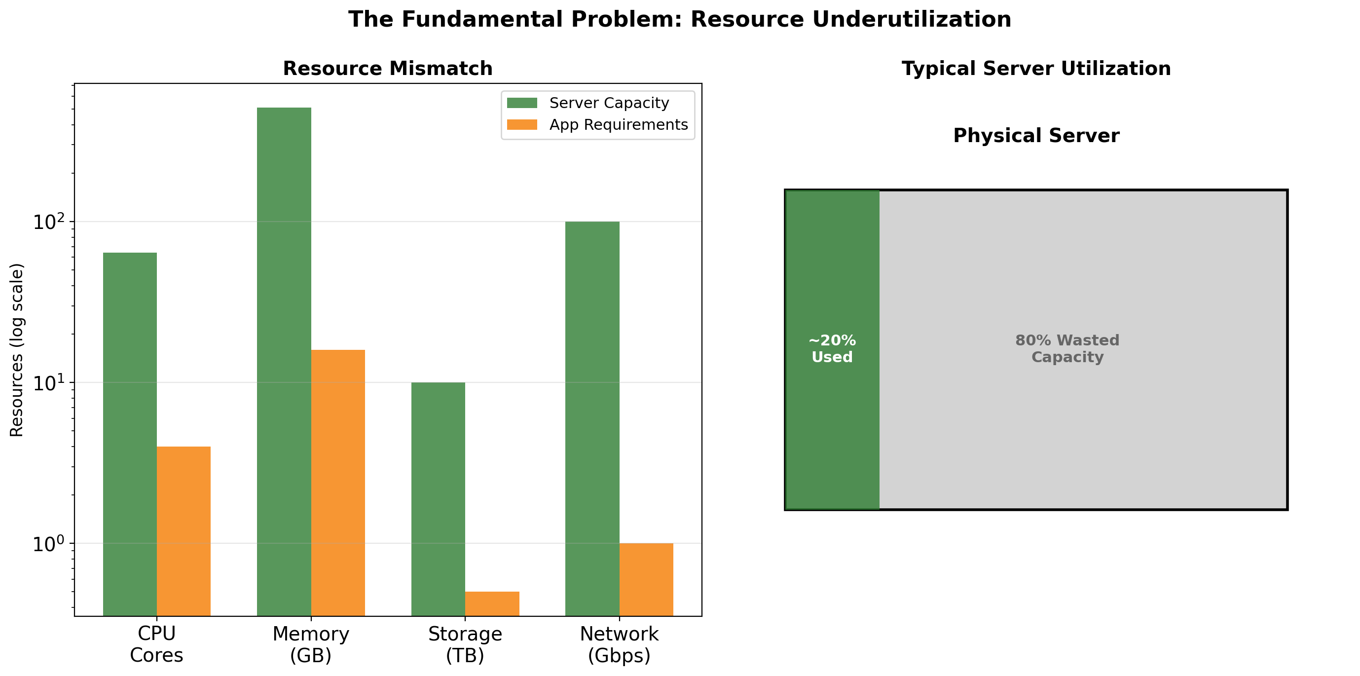
Dedicated Servers Sit Mostly Idle
If each component runs on its own physical server, utilization is typically 10-20%.
Why so low?
Servers are sized for peak load, not average load. The database server needs enough CPU to handle the traffic spike at 9am Monday. The rest of the week, most of that capacity sits unused.
Traffic patterns are bursty. A request takes 50ms of CPU time, then the server waits for the next request. Even under “heavy load,” CPUs spend most cycles waiting.
Redundancy requires spare capacity. If one app server fails, others must absorb its traffic. That headroom exists as idle capacity during normal operation.
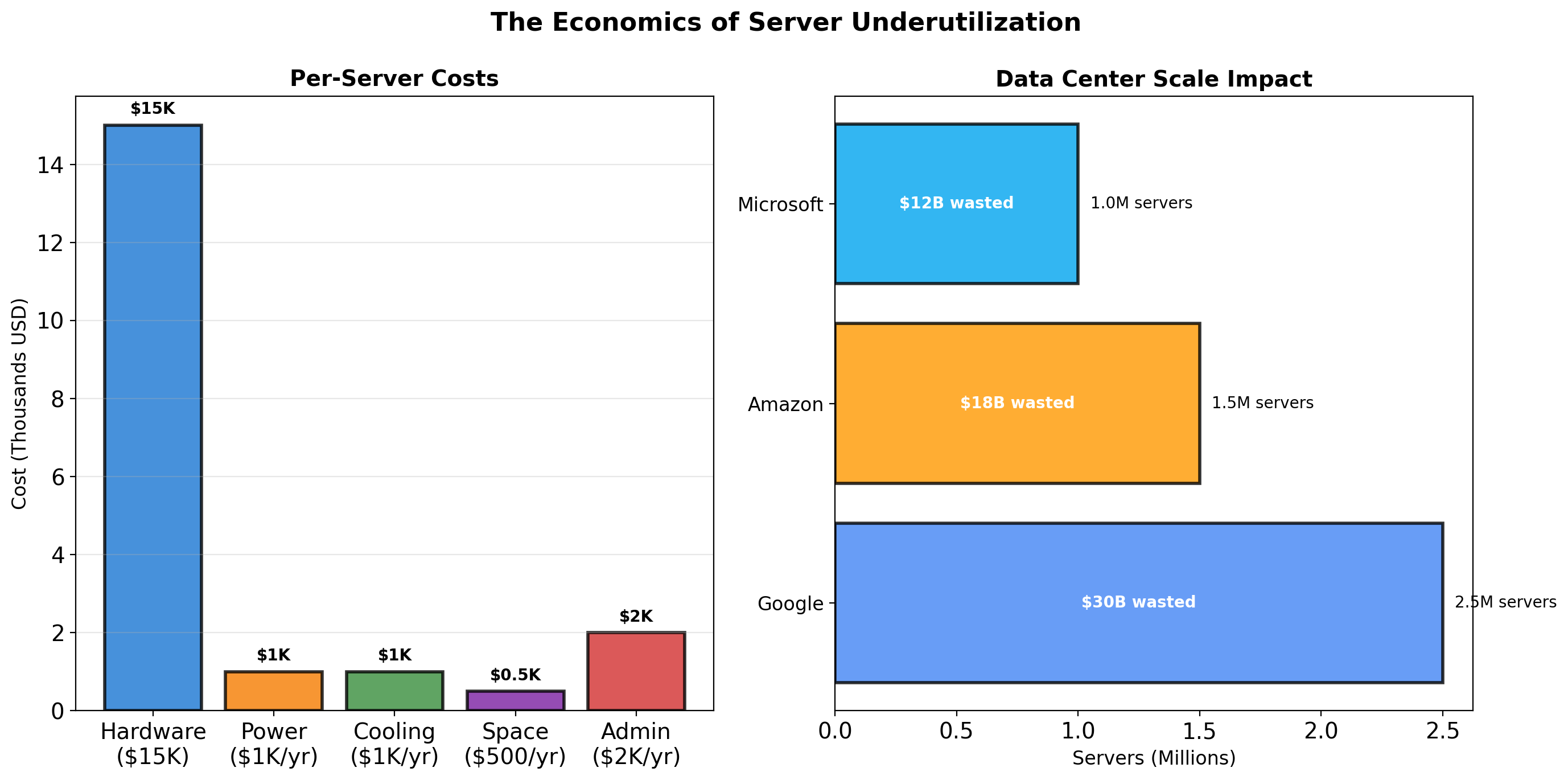
The Cost of Idle Hardware
A mid-range server costs approximately:
| Component | Cost |
|---|---|
| Server hardware | $8,000 - $15,000 |
| Amortized over 3-4 years | ~$250/month |
| Power (400W × 24/7) | ~$35/month |
| Cooling (40% of power) | ~$14/month |
| Rack space, networking | ~$50/month |
| Total cost of ownership | ~$350/month |
At 15% average utilization, the effective cost is:
\[\frac{\$350/\text{month}}{0.15} = \$2,333/\text{month per utilized server-equivalent}\]
Five physical servers doing the work of less than one.
At datacenter scale—thousands of servers—this waste represents millions of dollars annually. The economic pressure to improve utilization drove the development of virtualization technology.
Running Multiple Applications on One Server
The obvious solution: put multiple applications on the same physical server.
If each application averages 15% utilization, four applications together might achieve 50-60% utilization. Better economics.
But applications share more than hardware—they share the operating system. This creates problems.
Dependency Conflicts Break Co-located Applications
Application A is a legacy system written in 2019.
- Requires Python 3.7
- Uses
requestslibrary version 2.22 - Depends on OpenSSL 1.1.1
Application B is a new service deployed this year.
- Requires Python 3.11
- Uses
requestslibrary version 2.31 - Depends on OpenSSL 3.0
Both cannot run on the same OS installation. Python 3.7 and 3.11 have incompatible syntax. OpenSSL 1.1.1 and 3.0 have incompatible ABIs.
Virtual environments help with Python packages but not with system libraries. The OpenSSL conflict has no clean solution without OS-level isolation.
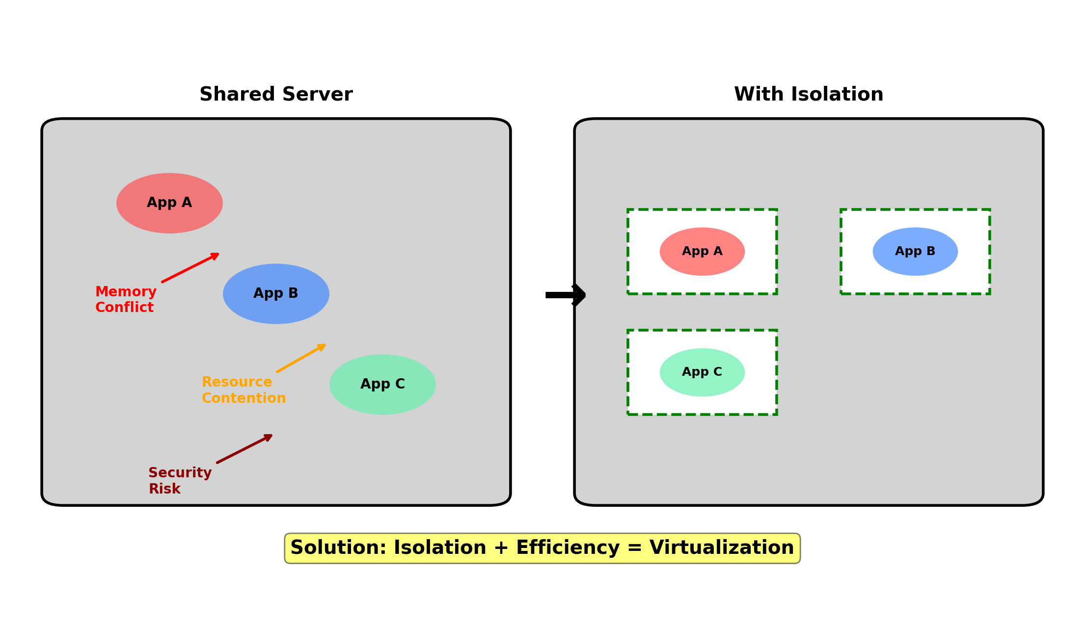
Resource Contention Affects All Applications
Applications on the same OS compete for resources without isolation.
Memory pressure
Application A has a memory leak. It slowly consumes available RAM. The OS starts swapping. Application B—completely unrelated—slows to a crawl because its memory pages are on disk.
CPU starvation
Application A enters a busy loop due to a bug. It consumes 100% of available CPU. Application B cannot process requests—no CPU cycles available.
Disk I/O saturation
Application A performs a bulk data export, writing gigabytes to disk. Application B’s database queries slow down—the disk is busy serving A’s writes.
The OS provides no mechanism to prevent one application from affecting another. They share a single pool of resources.
Security Boundaries Do Not Exist
Applications on the same OS can access each other’s data.
Filesystem access
Application A stores API keys in /etc/app-a/secrets.conf. Application B, running as the same user, can read that file. A vulnerability in B exposes A’s credentials.
Process visibility
Application A can list all processes with ps aux. It sees Application B’s command-line arguments, which might include database passwords.
Network access
Application A can bind to any port. It could intercept traffic meant for Application B by binding to B’s port first (if B restarts).
Shared users and permissions
If both run as www-data, they have identical filesystem permissions. Compromising one means compromising both.
Operational Coupling Creates Cascading Failures
OS updates affect all applications
A kernel security patch requires a reboot. All five applications go down simultaneously. Coordinating maintenance windows across unrelated teams becomes a scheduling nightmare.
One crash can affect others
Application A triggers a kernel panic (bad driver, memory corruption). All applications on that server die. Unrelated services suffer an outage.
Restart order matters
Application A starts before Application B. A grabs port 8080. B, which was supposed to use 8080, fails to start. Manual intervention required.
Log and metric confusion
All applications write to /var/log. Disk fills up—whose logs are responsible? System metrics show high CPU—which application is the cause?
Before Isolation Mechanisms: Networking
Isolated components still need to communicate. A database in its own isolated environment is useless if applications cannot query it.
Understanding how processes communicate over networks is prerequisite to understanding:
- How virtual machines present virtual network interfaces
- How containers isolate network namespaces
- How port mapping connects isolated containers to the outside world
- How services discover each other
Networking is not the focus of this course. But the basic model—processes binding to ports, TCP connections, request/response patterns—underpins everything that follows.
A Process Listens on a Port
A web server starts and binds to port 80.
import socket

server = socket.socket(socket.AF_INET, socket.SOCK_STREAM)
server.bind(('0.0.0.0', 80))
server.listen(5)

while True:
    client, addr = server.accept()
    # handle request
The process tells the operating system: “Send me any TCP traffic that arrives on port 80.”
The OS maintains a table mapping ports to processes. When a packet arrives destined for port 80, the kernel delivers it to this process.
Port numbers range from 0-65535. Ports below 1024 require elevated privileges (root/admin) on most systems.
Ports Multiplex Traffic to a Single Machine
A server has one IP address, but runs many network-facing processes. The web server, database, cache, and SSH daemon all need to receive traffic.
The problem: When a packet arrives at 192.168.1.10, which process should receive it?
The solution: Port numbers. Each packet carries a destination port. The OS uses this to route traffic to the correct process.
A port is an address within a machine. The IP address gets the packet to the right machine. The port gets it to the right process.
Destination: 192.168.1.10:5432
             └─────┬─────┘ └┬─┘
              machine     process
The combination of IP address and port uniquely identifies a network endpoint.
Multiple Processes Use Different Ports
A single machine can run many network services. Each binds to a different port.
| Port | Service | Protocol |
|---|---|---|
| 22 | SSH | Remote shell access |
| 80 | HTTP | Unencrypted web traffic |
| 443 | HTTPS | Encrypted web traffic |
| 5432 | PostgreSQL | Database queries |
| 6379 | Redis | Cache operations |
| 8080 | Application | Common alternative HTTP |
Only one process can bind to a given port. If nginx is listening on port 80, no other process can bind to 80. Attempting to do so returns “Address already in use.”
This constraint becomes important with containers: two containers both wanting port 80 on the same host need a resolution mechanism.
Clients Connect to Address and Port
To communicate with a service, a client needs two pieces of information:
IP address — identifies the machine
Port — identifies the process on that machine
import socket

client = socket.socket(socket.AF_INET, socket.SOCK_STREAM)
client.connect(('192.168.1.10', 5432))
client.send(b'SELECT * FROM users')
response = client.recv(4096)
The combination 192.168.1.10:5432 fully specifies the destination.
The client also uses a port—the OS assigns an arbitrary unused port (ephemeral port, typically 49152-65535) for the client side of the connection.
TCP Provides Reliable, Ordered Delivery
TCP (Transmission Control Protocol) handles complexity that applications shouldn’t deal with:
Reliable delivery
If a packet is lost, TCP retransmits it. The sender doesn’t receive acknowledgment within a timeout, so it sends again. The application sees reliable delivery without knowing about the loss.
Ordered delivery
Packets may arrive out of order due to network routing. TCP buffers and reorders them. The application receives bytes in the order they were sent.
Flow control
If the receiver is slow, TCP tells the sender to slow down. Prevents overwhelming the receiver’s buffers.
Connection-oriented
A connection is established before data transfer. Both sides know the other is present and ready.
TCP Costs: Latency and Overhead
TCP’s guarantees come at a cost.
Connection setup
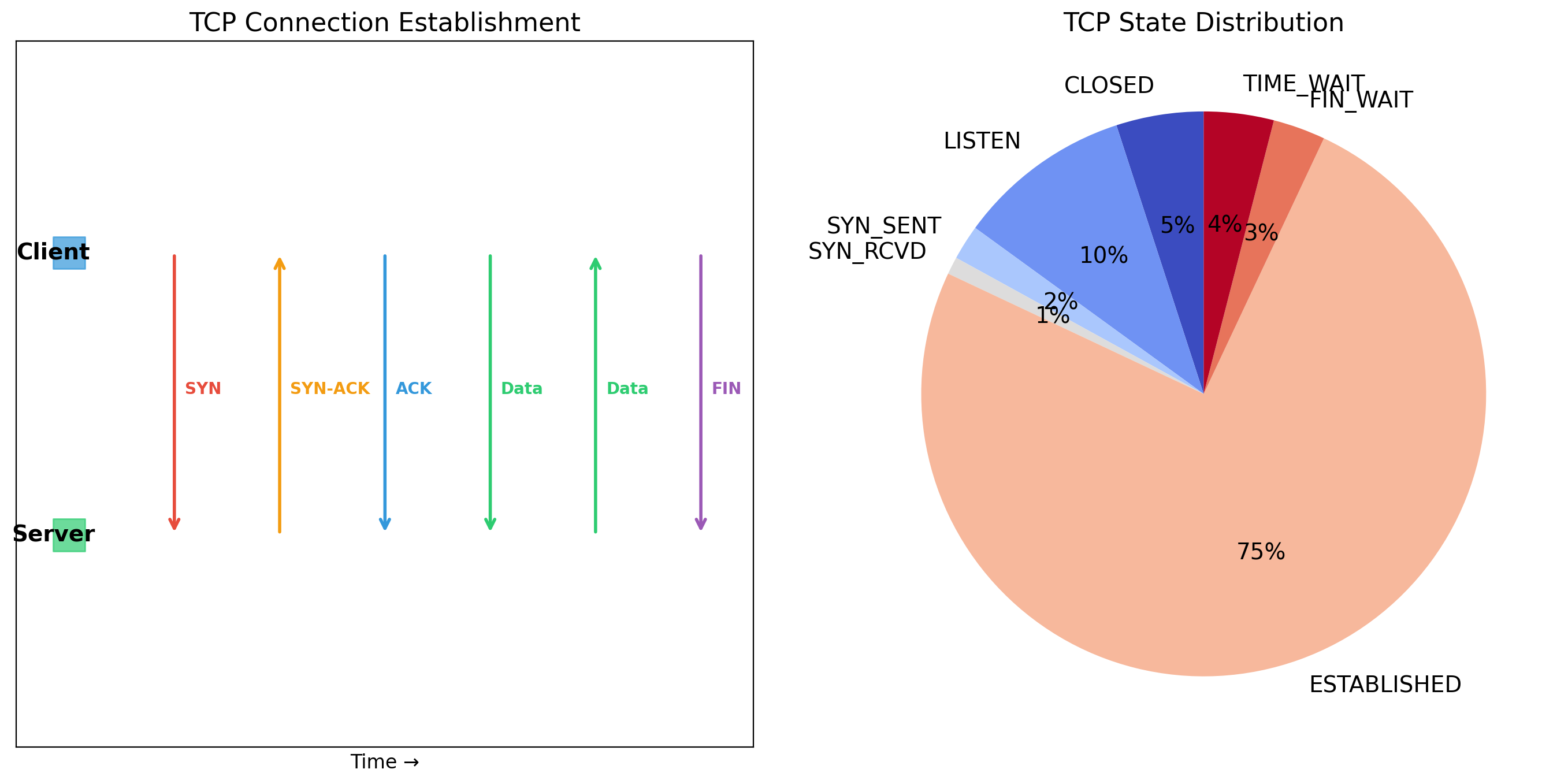
Before sending data, TCP performs a three-way handshake:
- Client sends SYN
- Server responds SYN-ACK
- Client sends ACK
One round-trip before any application data flows. For a server 50ms away, that’s 50ms of latency before the request even starts.
Head-of-line blocking
If packet 3 arrives before packet 2, TCP buffers packet 3 and waits. The application cannot see packet 3 until packet 2 arrives. Lost packet 2 blocks everything behind it.
Overhead
Every packet has a TCP header (20 bytes minimum). Acknowledgments consume bandwidth. Retransmission timers consume memory.
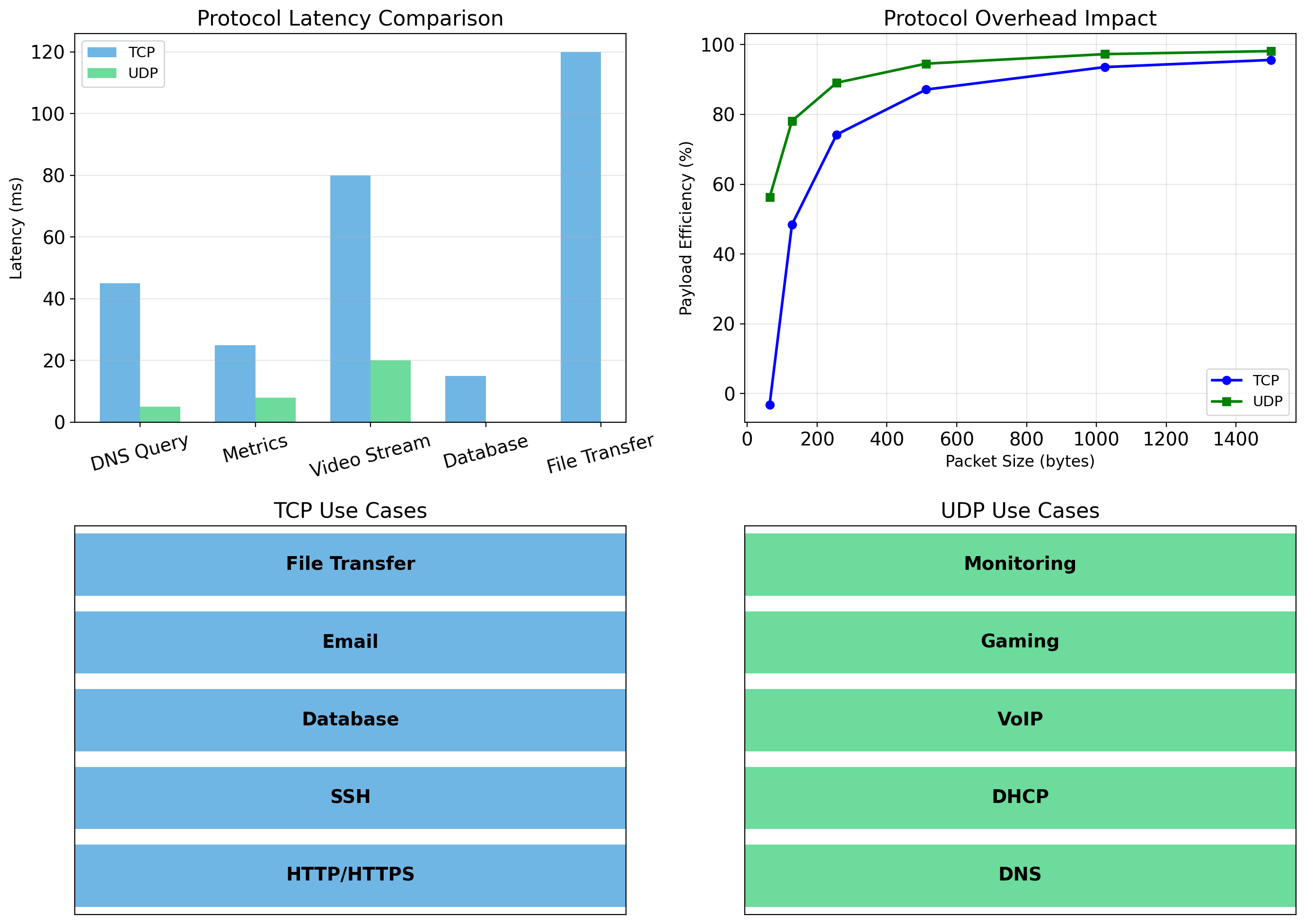
For most application traffic—HTTP requests, database queries, API calls—TCP’s guarantees are worth the cost. You want your database query to arrive complete and in order.
UDP: Unreliable but Fast
UDP (User Datagram Protocol) provides minimal service:
No connection setup
Send packets immediately. No handshake required.
No reliability
Packets may be lost. UDP does not retransmit.
No ordering
Packets may arrive out of order. UDP does not reorder.
No flow control
Sender can overwhelm receiver. UDP does not slow down.
Why use UDP?
When speed matters more than reliability. When the application handles reliability itself. When occasional loss is acceptable.
Video streaming: a dropped frame is better than pausing for retransmission. DNS queries: simple request/response, application can retry if needed.
Network Layers Separate Responsibilities
Network communication is organized into layers, each handling a specific responsibility:
Application layer
Your code. HTTP requests, database queries, API calls. Deals with application-level semantics.
Transport layer
TCP or UDP. Handles reliability (or not), port multiplexing, connection management. Delivers data to the right process.
Network layer
IP. Handles addressing and routing. Gets packets from source machine to destination machine across potentially many intermediate routers.
Link layer
Physical delivery on a local network segment. Ethernet, WiFi. Gets frames to the next hop.
Each layer uses the services of the layer below without knowing its implementation details.
Your Code Lives at the Application Layer
When your application sends an HTTP request:
response = requests.get('http://api.example.com/users')You don’t specify:
- How to establish a TCP connection
- How to handle packet loss
- How to route to
api.example.com - Which network interface to use
The layers below handle all of that. Your application layer code expresses intent: “GET the resource at this URL.” The transport layer establishes a reliable connection. The network layer routes packets to the destination. The link layer transmits frames on the wire.
This separation means your application code works regardless of whether you’re on WiFi, Ethernet, or a mobile network.
IP Addresses Identify Machines
Every machine on a network has an IP address.
IPv4 addresses
Four numbers 0-255, separated by dots: 192.168.1.10
32 bits total, approximately 4.3 billion possible addresses. Running out—most of the public address space is allocated.
IPv6 addresses
Eight groups of hexadecimal: 2001:0db8:85a3:0000:0000:8a2e:0370:7334
128 bits, effectively unlimited addresses. Adoption growing but IPv4 still dominates.
Private address ranges
10.0.0.0/8— 16 million addresses172.16.0.0/12— 1 million addresses192.168.0.0/16— 65,000 addresses
Not routable on the public internet. Used within organizations, home networks, cloud VPCs.
DNS Translates Names to Addresses
IP addresses are hard to remember. DNS (Domain Name System) provides human-readable names.
$ nslookup google.com
Name:    google.com
Address: 142.250.80.46
When your application connects to api.example.com:
- Application calls
getaddrinfo("api.example.com") - OS checks local cache
- If not cached, queries DNS resolver
- Resolver queries DNS hierarchy
- Returns IP address(es)
- Application connects to that IP
DNS records have TTL (time-to-live). Clients cache responses for that duration. Allows servers to change IP addresses—clients eventually get the new address.
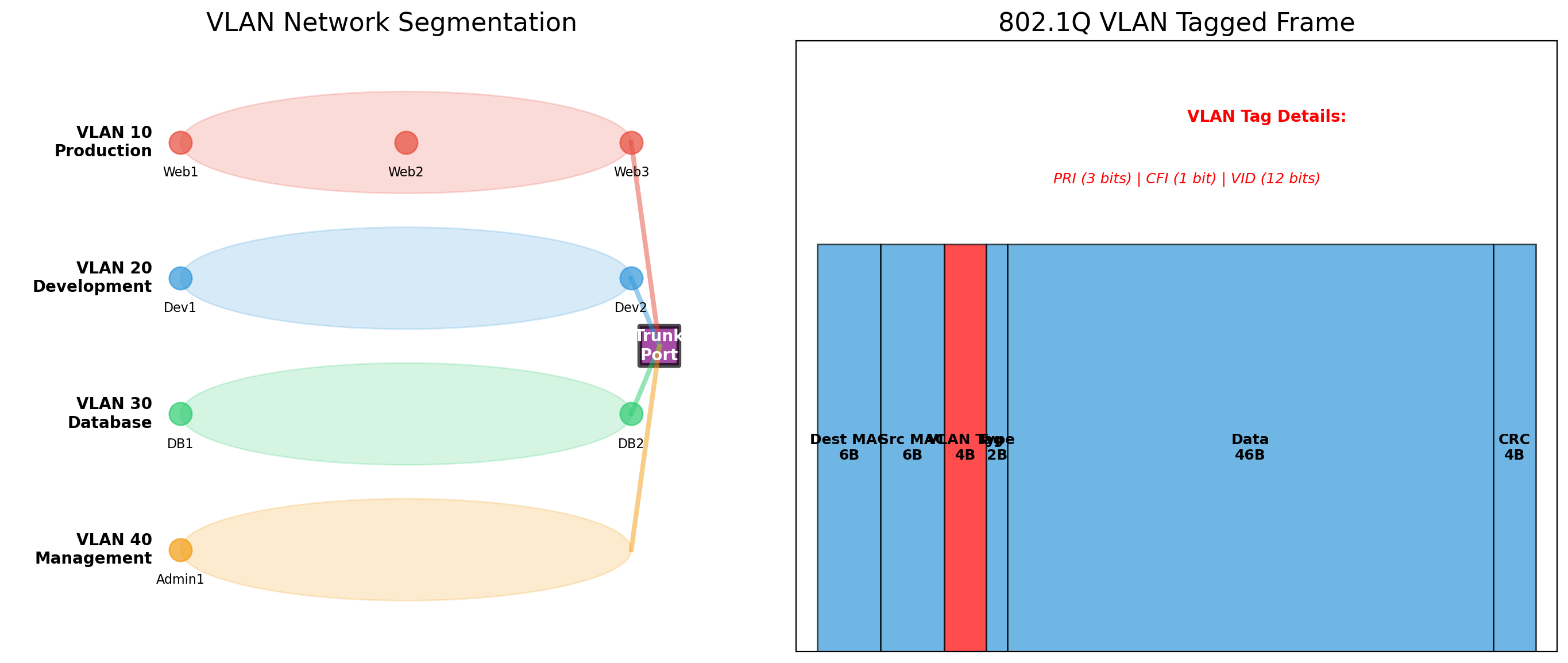
VLANs Provide Logical Network Separation
Physical networks can be logically partitioned using VLANs (Virtual Local Area Networks).
Without VLANs
All devices on a switch can communicate directly. The marketing department’s printers are on the same network as engineering’s servers.
With VLANs
The switch tags traffic with VLAN IDs. VLAN 10 traffic only reaches VLAN 10 ports. Marketing and engineering are isolated even though they share physical infrastructure.
Why this matters
- Security: Limit blast radius of compromised devices
- Performance: Reduce broadcast traffic
- Organization: Group devices logically, not physically
Cloud providers use similar concepts. AWS VPCs, Azure VNets—logical network isolation on shared physical infrastructure.
Dedicated Servers Waste Resources, Shared OS Creates Conflicts
Dedicated servers
Each workload gets its own machine. Complete isolation. But 10-20% utilization—85% of hardware sits idle.
Shared OS
Multiple workloads on one machine. Better utilization. But dependency conflicts, resource contention, security risks, coupled failures.
Neither option is acceptable at scale. Workloads need to:
- Run in separate environments
- Share underlying hardware
- Not interfere with each other
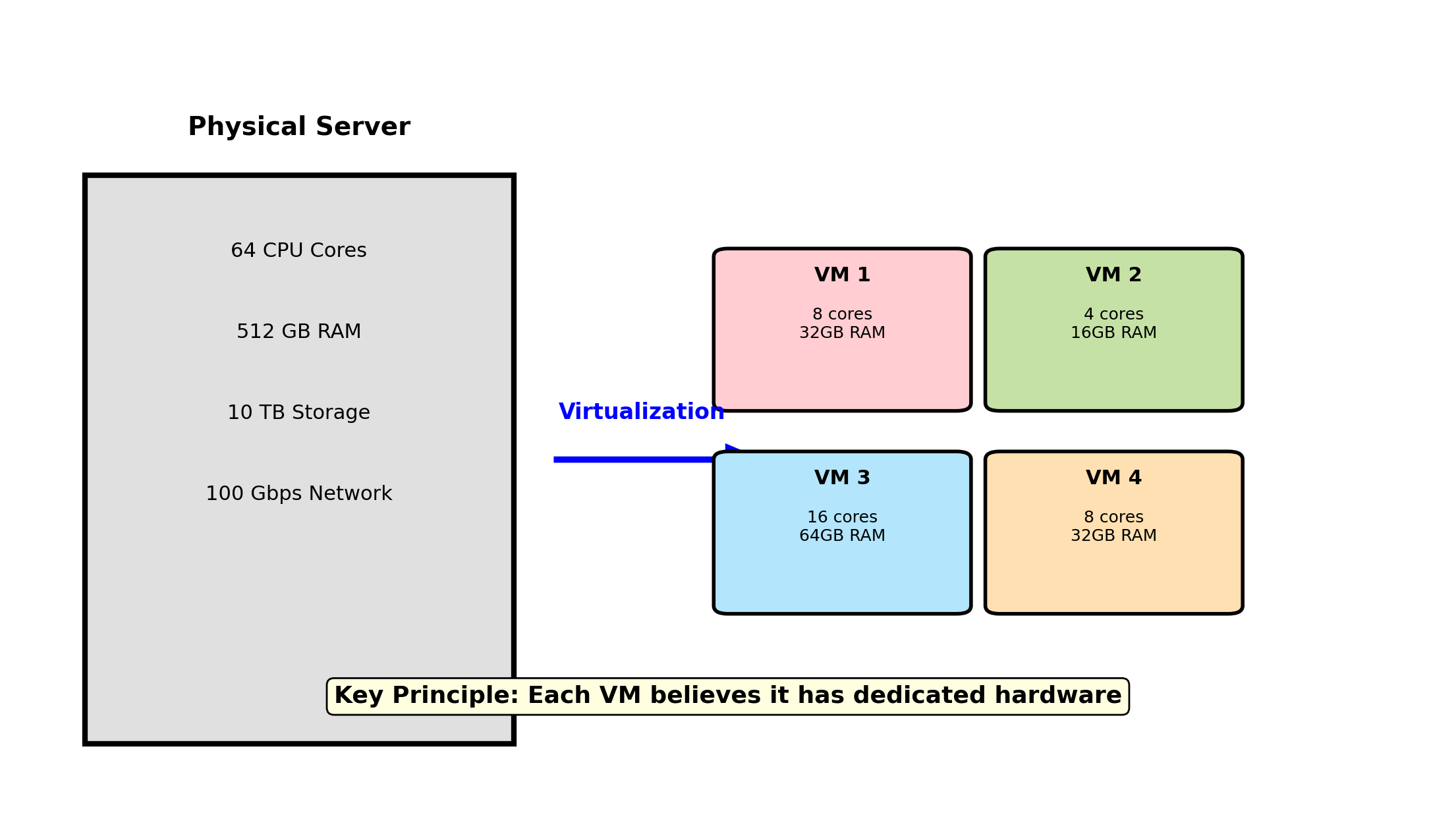
One Physical Machine, Multiple Virtual Machines
Each VM sees its own complete machine: CPU, memory, disk, network interfaces. The hypervisor divides physical resources among VMs and enforces isolation between them.
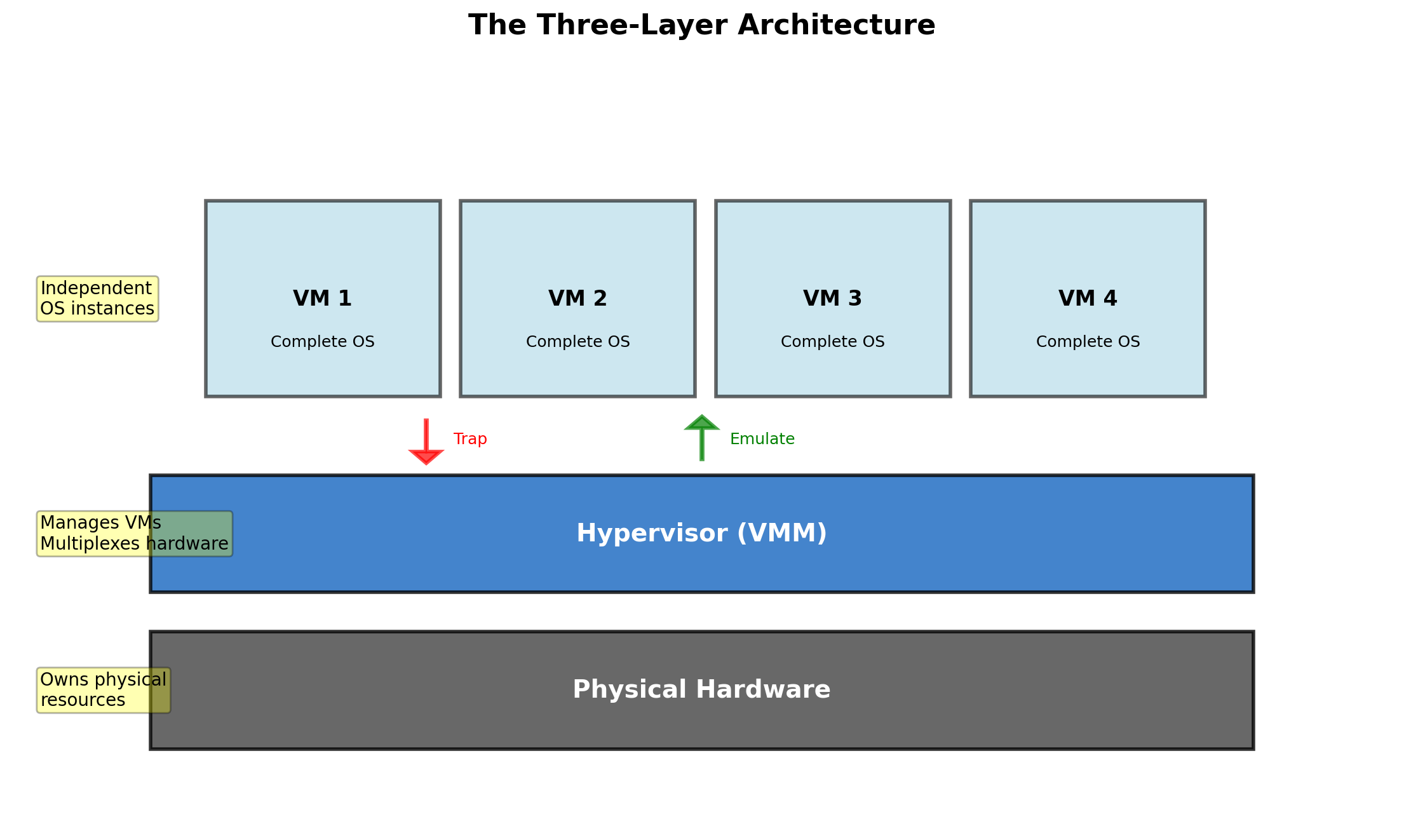
The Hypervisor Virtualizes Hardware
The hypervisor is a software layer that:
- Presents virtual hardware to each VM
- Schedules VM execution on physical CPUs
- Manages memory allocation across VMs
- Mediates access to physical devices
Each VM runs a full operating system. That OS believes it’s running on real hardware. The hypervisor maintains this illusion.
VMs cannot access each other’s memory, see each other’s processes, or interfere with each other’s operation. The hypervisor enforces these boundaries.
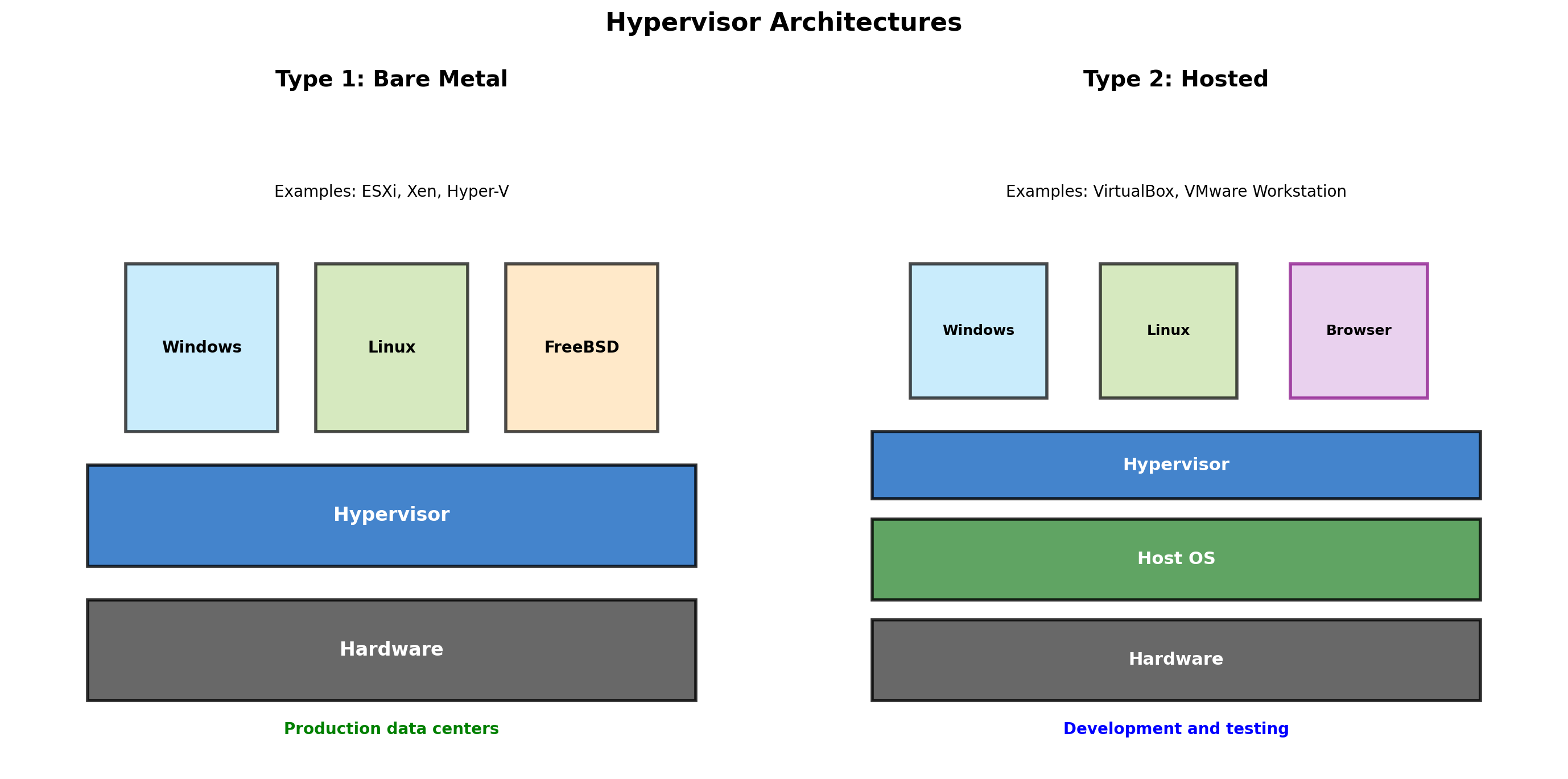
Type 1 Hypervisors Run on Bare Metal
Type 1 (bare metal)
The hypervisor runs directly on hardware. No host operating system underneath.
Examples:
- Xen — Powers AWS EC2
- VMware ESXi — Enterprise datacenters
- Microsoft Hyper-V — Windows Server
- KVM — Linux kernel module
Used in production environments where performance and isolation matter. The hypervisor is the operating system for the physical machine.
Type 2 Hypervisors Run on a Host OS
Type 2 (hosted)
The hypervisor runs as an application on a host operating system.
Examples:
- VirtualBox — Free, cross-platform
- VMware Workstation — Windows/Linux
- Parallels — macOS
- VMware Fusion — macOS
Used for development and desktop virtualization. Convenient—runs alongside normal applications. But an extra OS layer adds overhead.

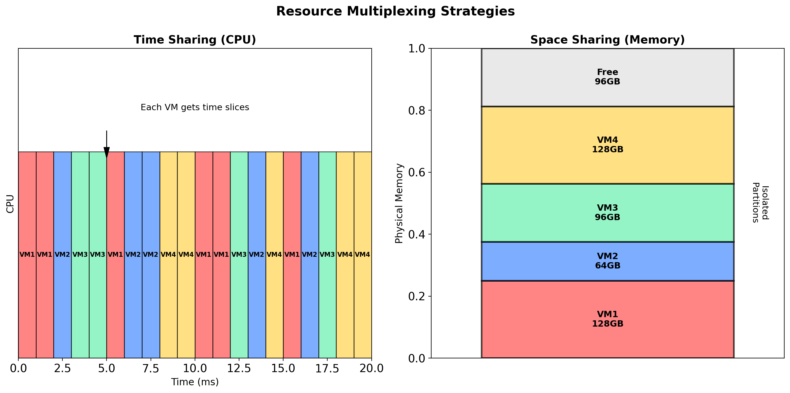
CPU Virtualization
Each VM has virtual CPUs (vCPUs). The hypervisor schedules vCPUs onto physical cores.
Time-slicing
With more vCPUs than physical cores, the hypervisor switches between VMs. Each VM gets a fraction of CPU time.
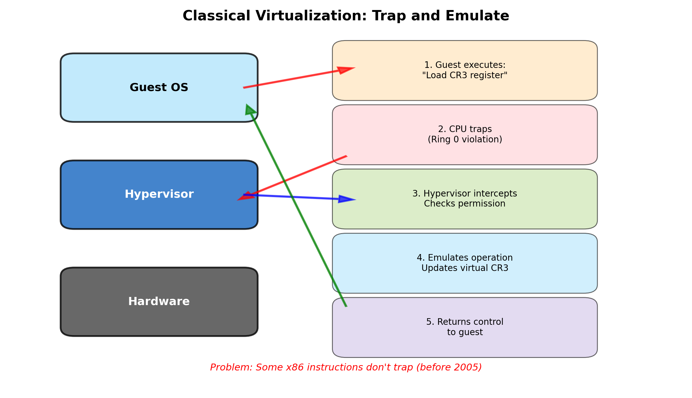
Hardware support
Modern CPUs include virtualization extensions (Intel VT-x, AMD-V). These allow the hypervisor to run guest OS code at near-native speed.
Without hardware support, the hypervisor must trap and emulate privileged instructions—significantly slower.
Overcommit
A 16-core server can run VMs with a total of 32+ vCPUs. Works if VMs aren’t all CPU-bound simultaneously.
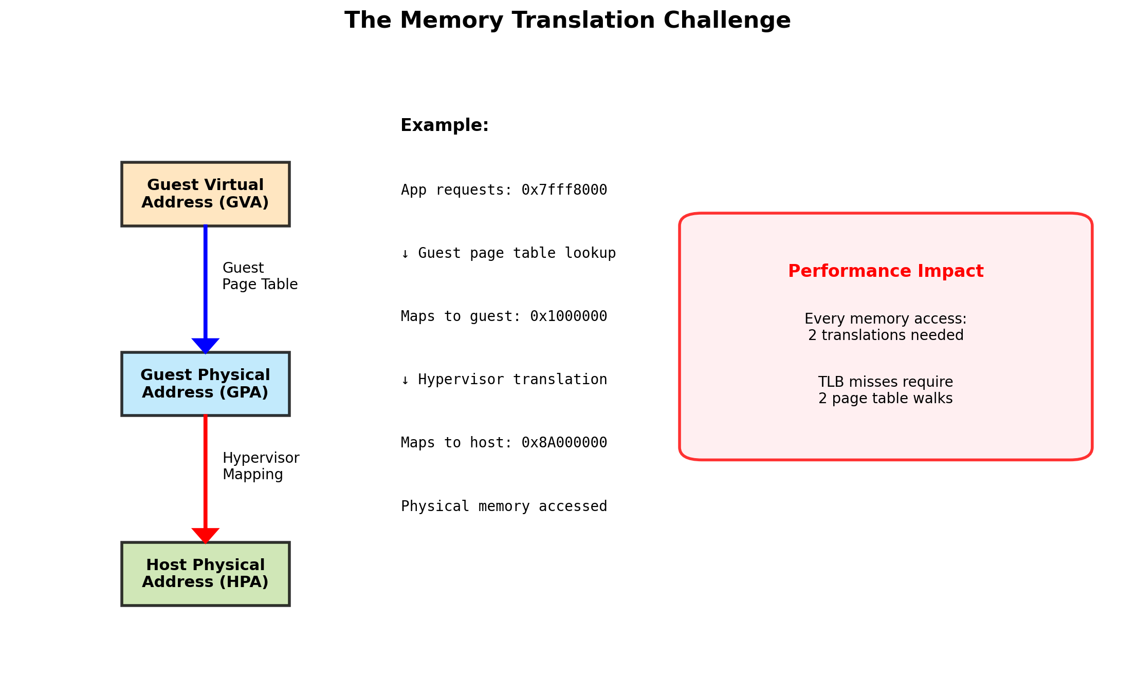
Memory Virtualization
Each VM sees contiguous physical memory starting at address 0. But the actual physical memory is elsewhere.
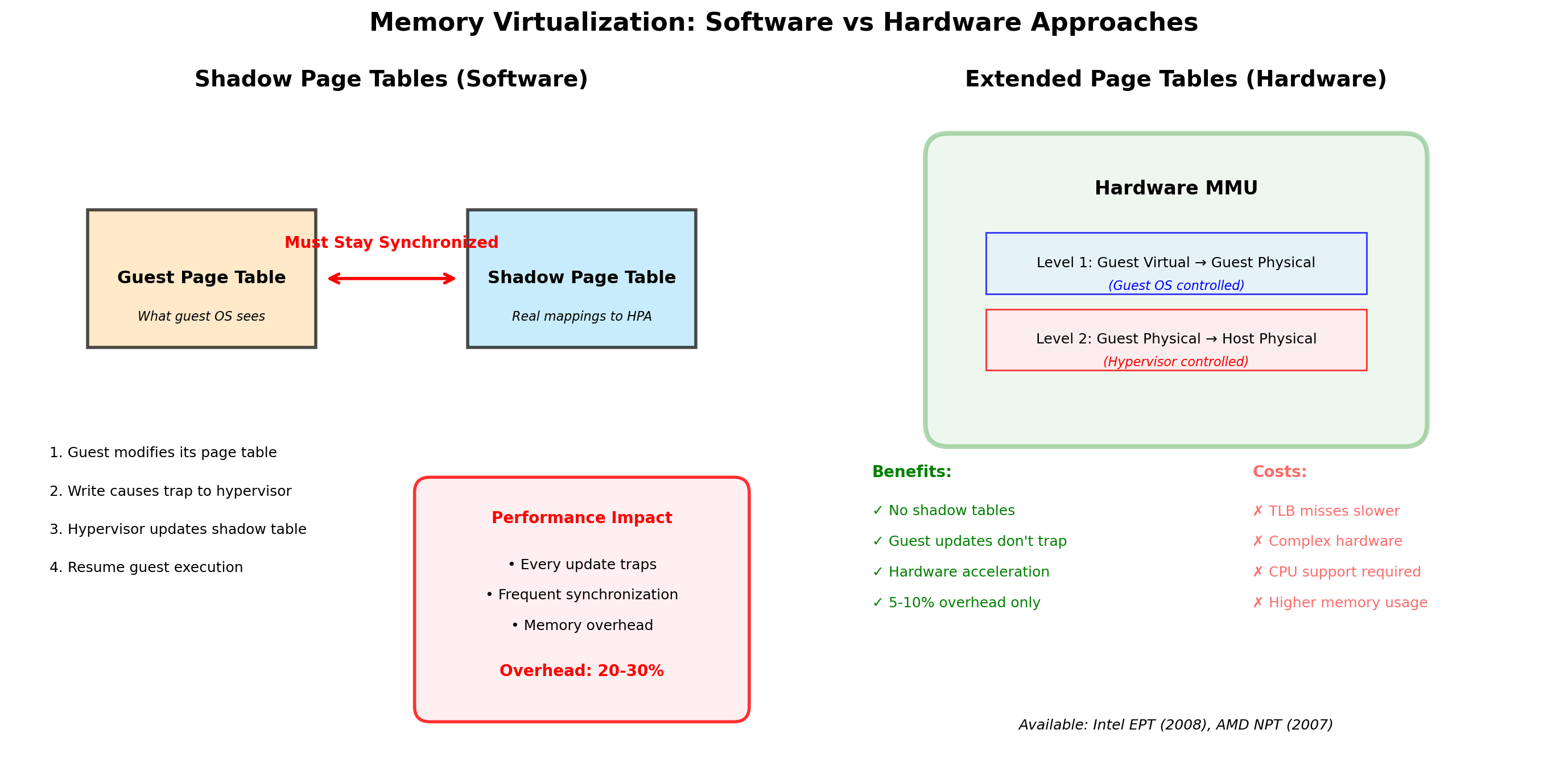
Two levels of translation
- Guest virtual → Guest physical (guest OS page tables)
- Guest physical → Host physical (hypervisor)
Hardware support (EPT/NPT)
Extended Page Tables (Intel) and Nested Page Tables (AMD) perform both translations in hardware. Without this, the hypervisor must intercept every memory access—extremely slow.
Isolation
VM 1’s guest physical address 0x1000 maps to a different host physical address than VM 2’s 0x1000. Neither can access the other’s memory. The CPU enforces this.
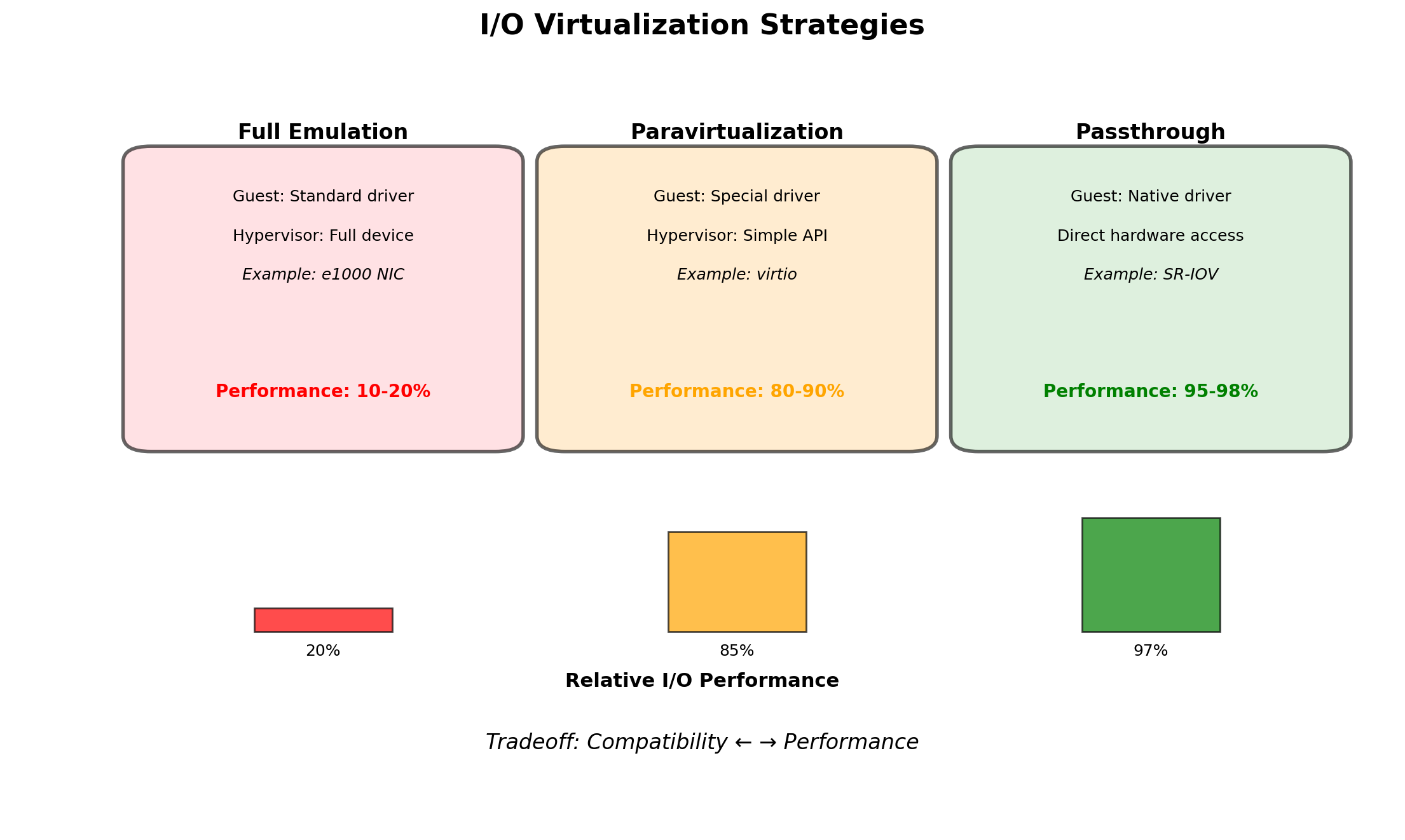
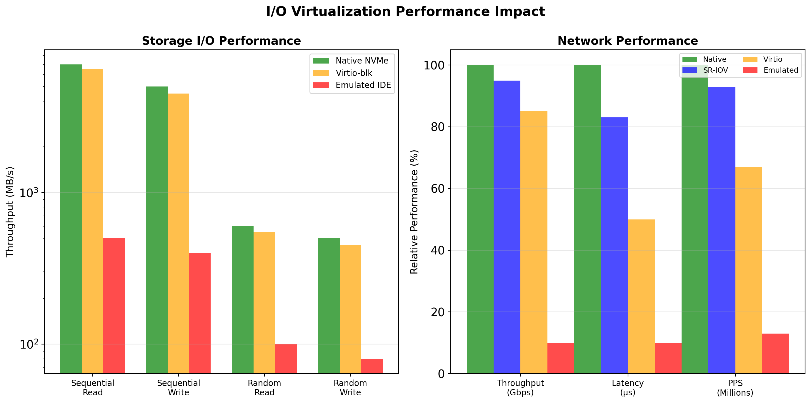
Storage and Network Virtualization
Virtual disks
Each VM sees disk devices (e.g., /dev/sda). These map to files on the host or raw disk partitions.
- VMDK, VHD, QCOW2 formats
- Thin provisioning: allocate space as used
- Snapshots: point-in-time copies
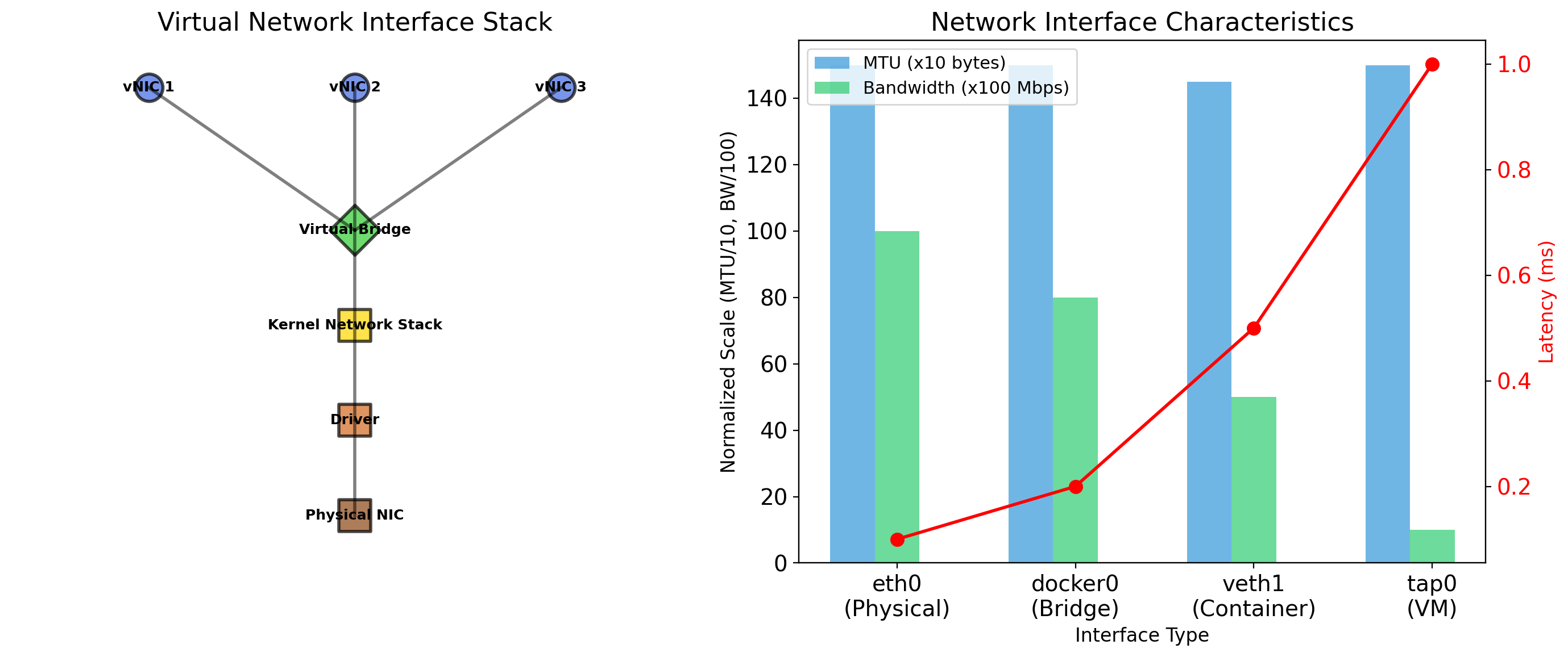
Virtual network interfaces
Each VM has virtual NICs. The hypervisor connects these to:
- Virtual switch — VMs communicate with each other
- Bridge — VMs appear on the physical network
- NAT — VMs share host’s IP for outbound traffic
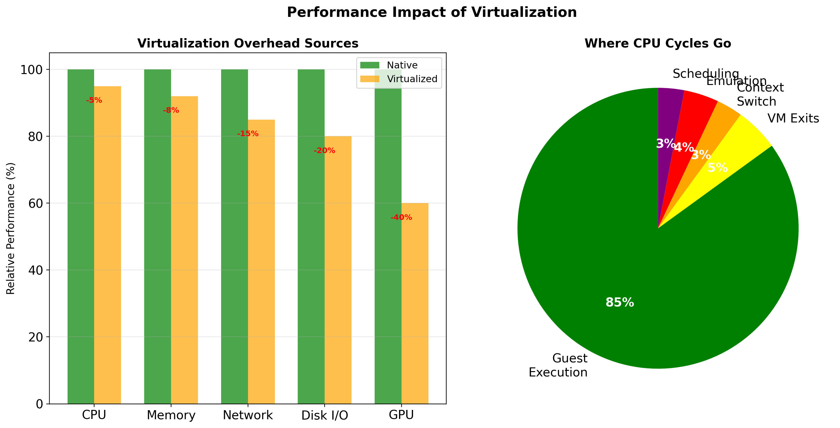
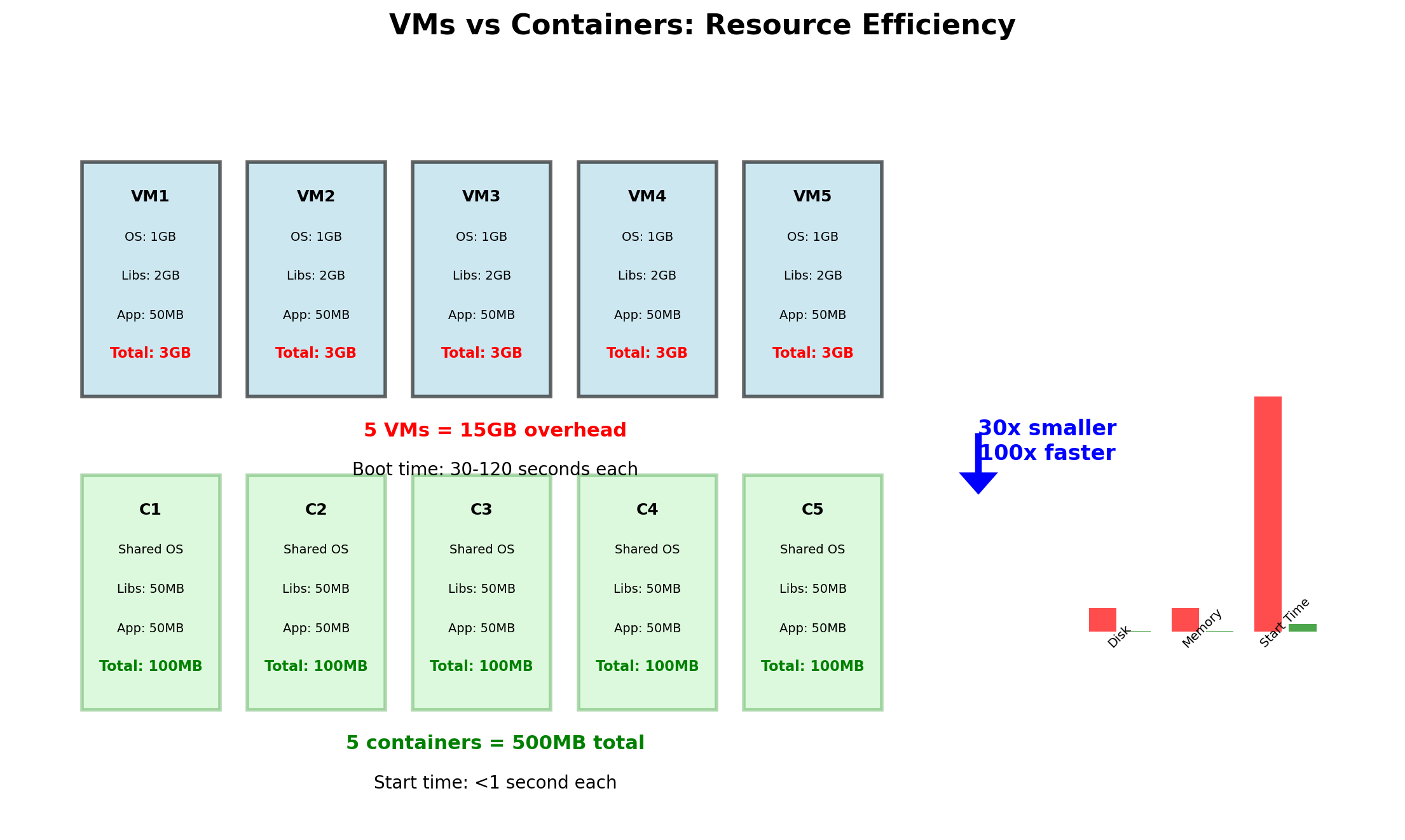
VM Overhead is Substantial
Each VM runs a complete operating system. This has costs:
| Resource | Per-VM Overhead |
|---|---|
| Memory | 512 MB - 2 GB for OS |
| Disk | 5 - 20 GB for OS install |
| Boot time | 30 seconds - 2 minutes |
| CPU | Hypervisor scheduling overhead |
10 VMs on a 256 GB server
- 10-20 GB consumed by OS memory
- 50-200 GB disk for OS installations
- 5-20 minutes total boot time
This overhead doesn’t do useful work. It’s the cost of isolation.
Cloud Instances Are Virtual Machines
When you launch an EC2 instance, you’re creating a VM.
aws ec2 run-instances \
  --instance-type t3.medium \
  --image-id ami-0abcdef1234567890
t3.medium specifies:
- 2 vCPUs
- 4 GB memory
- Burstable CPU credits
AWS runs a hypervisor (Nitro, based on KVM) on physical servers. Your instance is a VM on that hypervisor, alongside other customers’ VMs.
You don’t see the hypervisor. You see a complete machine with the resources you requested.
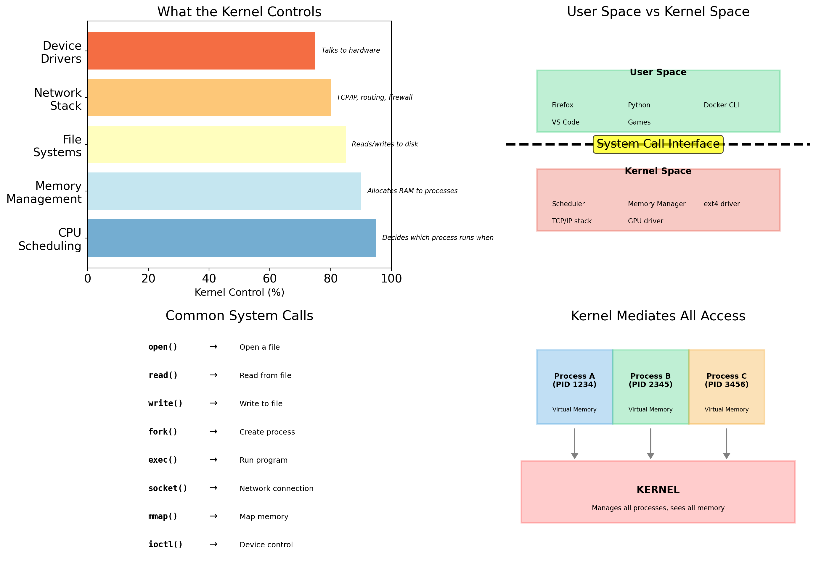
The Operating System Kernel
The kernel is the core of the operating system. It runs with full hardware privileges and manages:
Hardware access
CPU scheduling, memory allocation, disk I/O, network interfaces. Applications cannot touch hardware directly—they ask the kernel.
Process management
Starting, stopping, scheduling processes. Deciding which process runs on which CPU core.
Resource allocation
Which process gets how much memory. Which can access which files. Which can open network connections.
The kernel is the boundary between software and hardware. Everything else runs “on top of” the kernel.

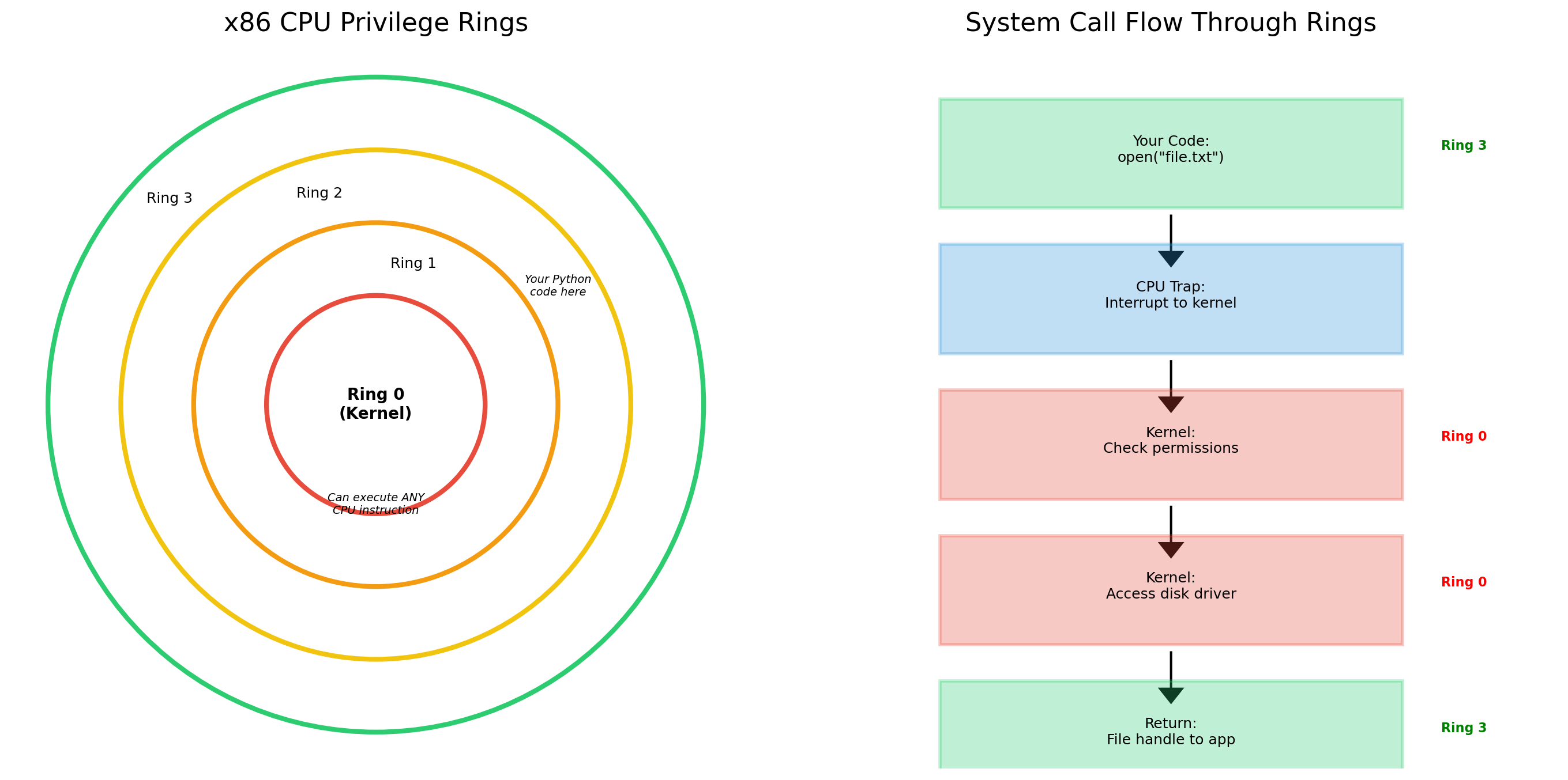
Processes Request Resources Through System Calls
When your application needs to:
- Open a file
- Allocate memory
- Send network data
- Start another process
It makes a system call to the kernel. The kernel validates the request, performs the operation, and returns the result.
# Your code
f = open('/data/users.json', 'r')

# What actually happens:
# 1. Python calls open()
# 2. open() makes syscall to kernel
# 3. Kernel checks permissions
# 4. Kernel opens file, returns handle
# 5. Your code gets file object
The application never touches the disk directly. The kernel mediates all access.
The Kernel Sees All Processes and Resources
On a normal Linux system, the kernel maintains:
One process table
Every process has an entry. Each can see other processes with ps aux.
One filesystem tree
Starting at /. All processes see the same files (subject to permissions).
One network stack
Shared IP addresses, ports, routing tables.
One set of users
UID 1000 is the same user for all processes.
When you run multiple applications, they all share these views. Process A can see process B. Both see the same /tmp. Both compete for the same ports.
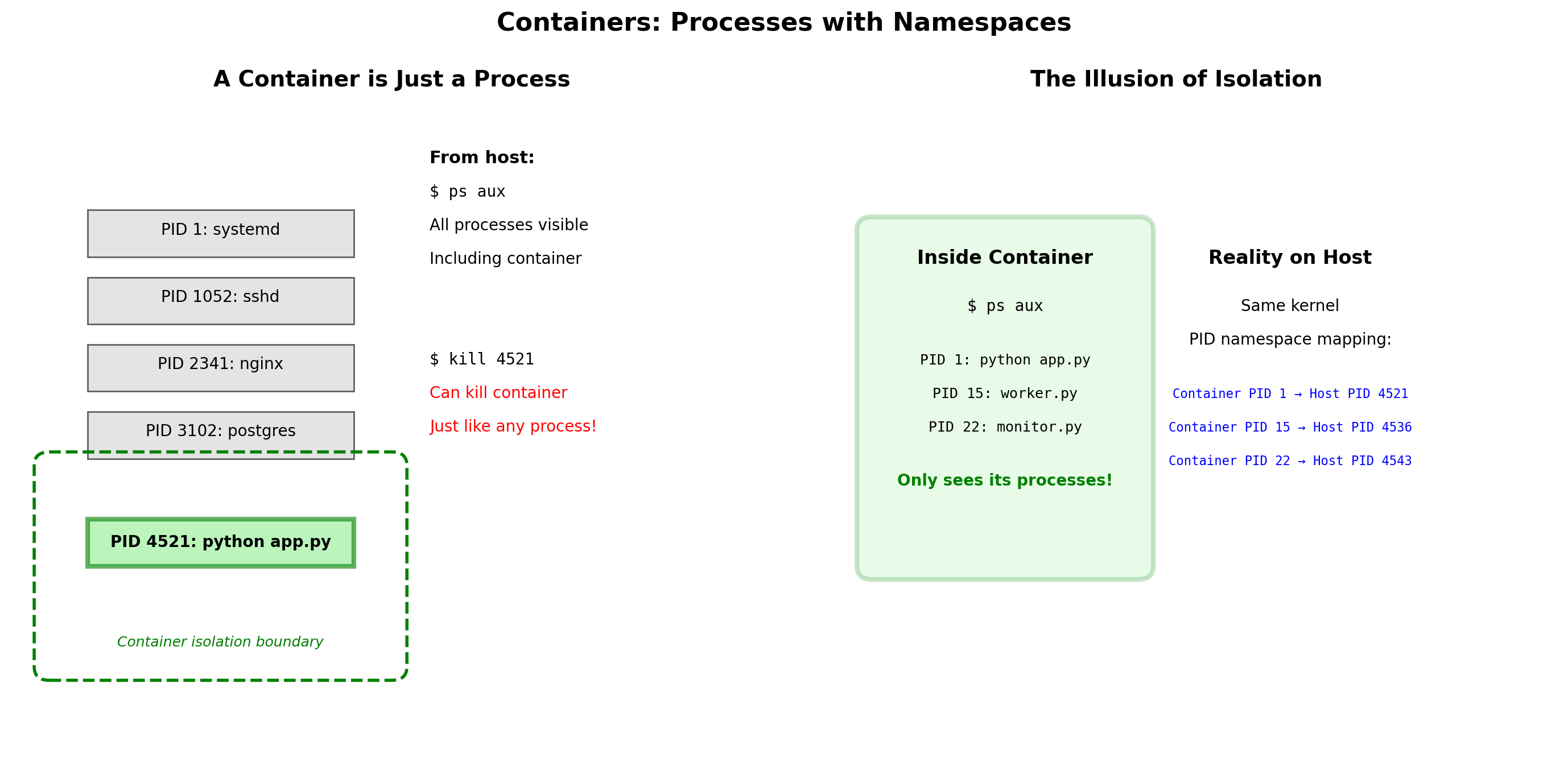
Containers: Processes with Restricted Kernel Views
A container is not a virtual machine. It does not run a separate kernel.
A container is a process (or group of processes) that the kernel treats specially. When a containerized process asks “what processes exist?”, the kernel returns a filtered answer.
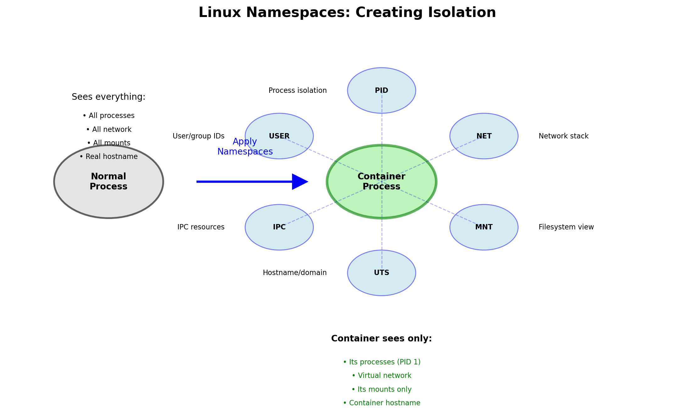
The kernel provides namespaces—separate views of system resources. A process in a namespace sees only what that namespace contains.
Same kernel. Different perspectives.
The containerized process believes it’s alone on the system. It sees only its own processes, its own filesystem, its own network stack. The kernel maintains this illusion.
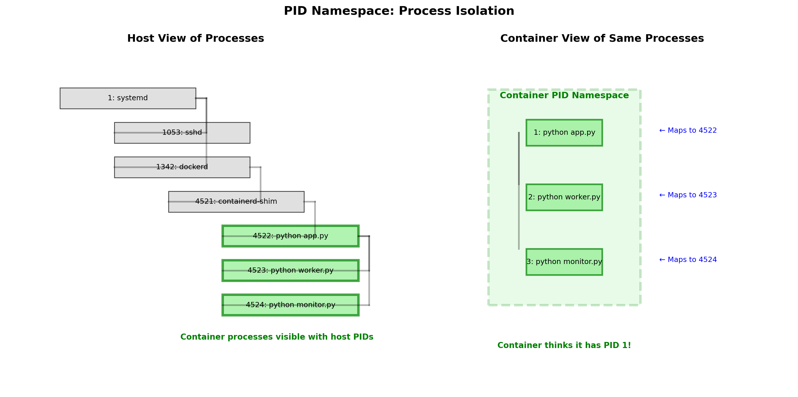
PID Namespace: Isolated Process Trees
Each container has its own process ID namespace.
Inside the container:
The main process is PID 1. Child processes are PID 2, 3, etc. The container sees only its own processes.
On the host:
The same processes have different PIDs. Container A’s PID 1 might be host PID 4523.
# Inside container
$ ps aux
PID  COMMAND
1    /app/server
2    /app/worker

# On host
$ ps aux | grep app
4523  /app/server   # Container A's PID 1
4524  /app/worker   # Container A's PID 2
Container A cannot see or signal Container B’s processes. They exist in separate PID namespaces.
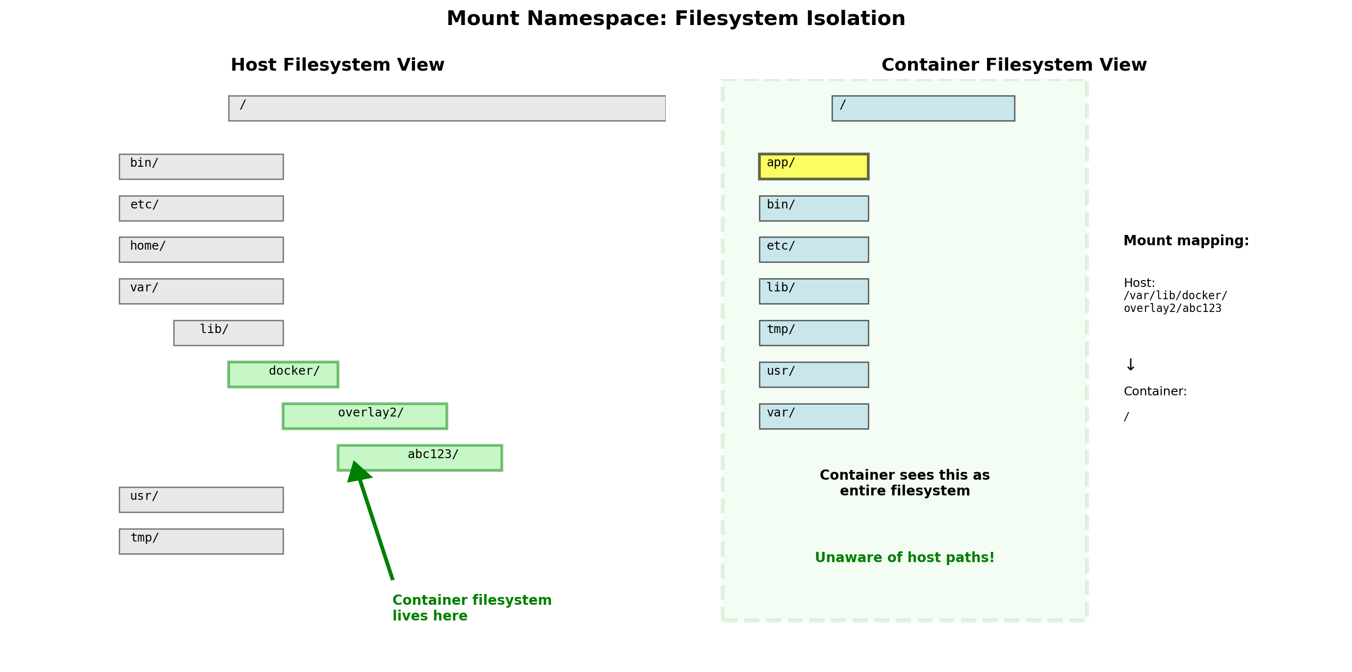
Mount Namespace: Isolated Filesystem Views
Each container has its own mount namespace—a separate view of the filesystem.
Container sees its own root
The container’s / is not the host’s /. It’s a separate directory tree, typically from a container image.
# Container A
$ ls /
bin  etc  home  lib  usr  app

# Container B (different image)
$ ls /
bin  etc  lib64  opt  usr  data

# Host
$ ls /
bin  boot  dev  etc  home  lib  ...
Container A cannot see Container B’s files. Neither can see arbitrary host files. The kernel enforces this separation.
Host directories can be explicitly mounted into containers when needed—but the default is isolation.
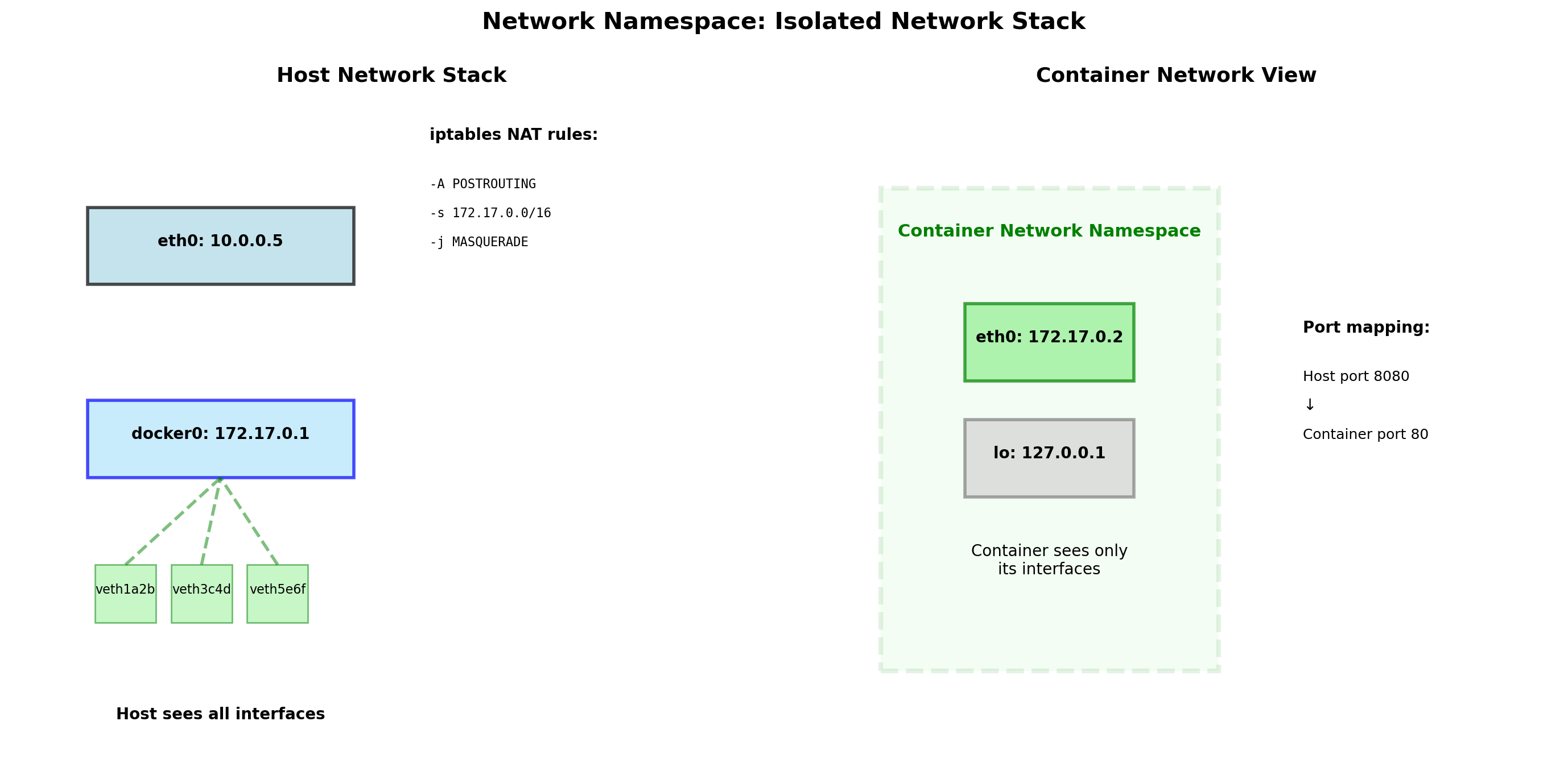
Network Namespace: Isolated Network Stacks
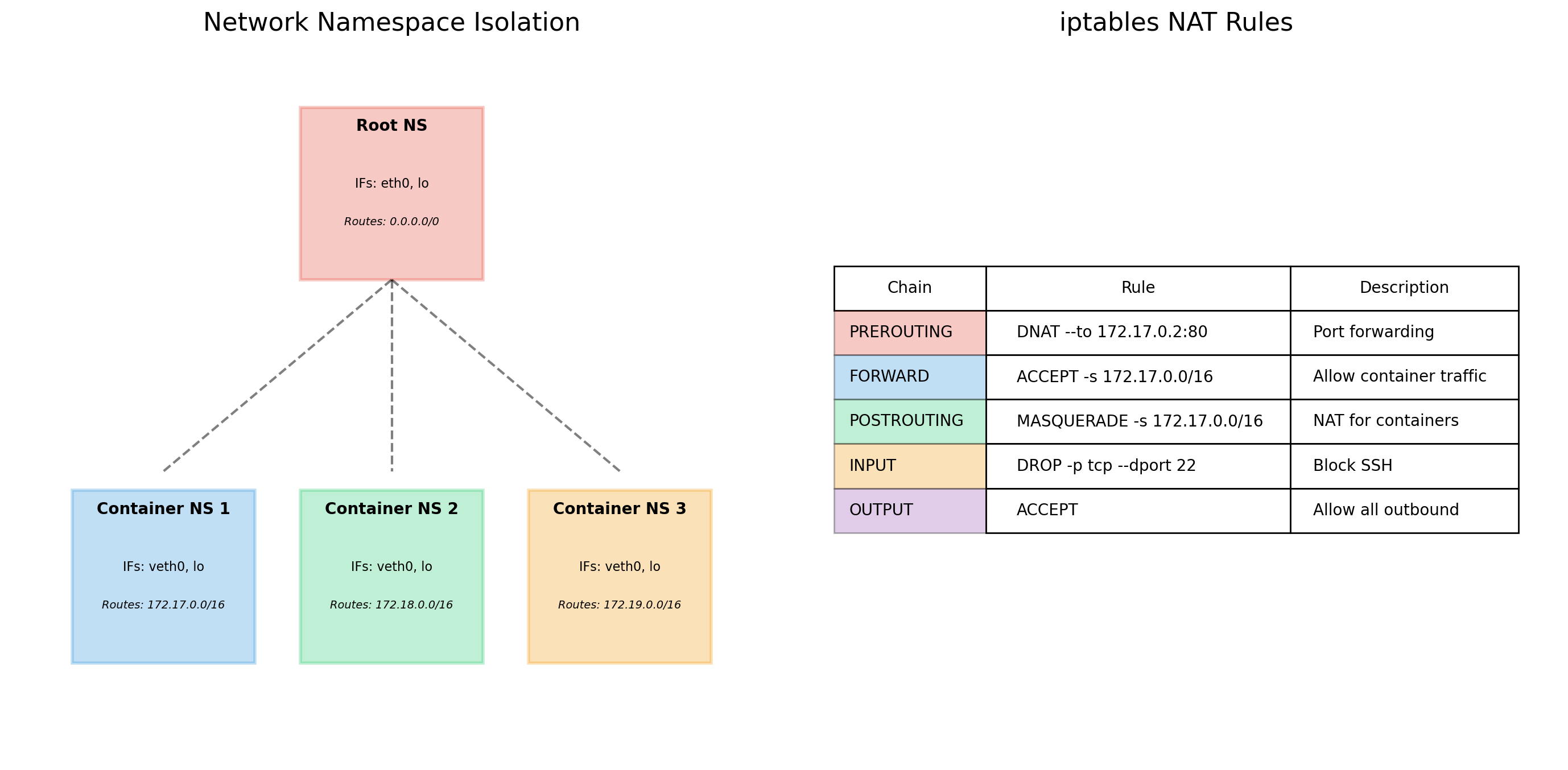
Each container has its own network namespace:
- Own network interfaces
- Own IP addresses
- Own routing tables
- Own port space
Port conflicts eliminated
Container A listens on port 80. Container B also listens on port 80. No conflict—each has its own port namespace.
# Container A
$ ip addr
eth0: 172.17.0.2/16

# Container B
$ ip addr
eth0: 172.17.0.3/16

# Both listen on :80, no conflict
The host bridges container networks to the physical network. Containers can communicate with each other and the outside world through this bridge.
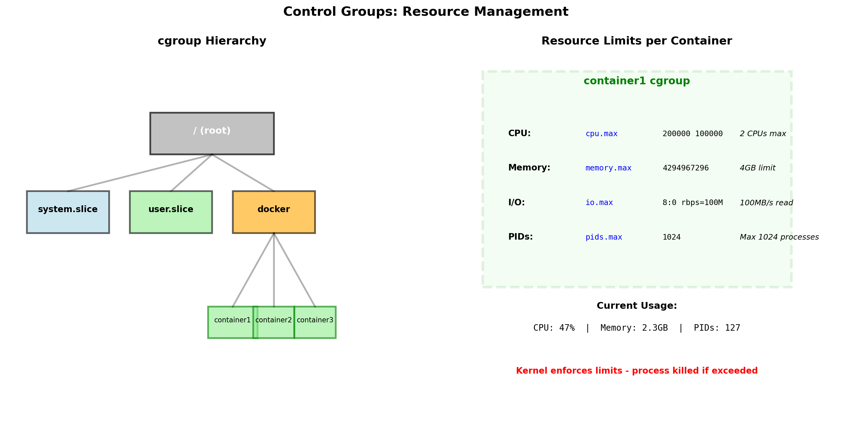
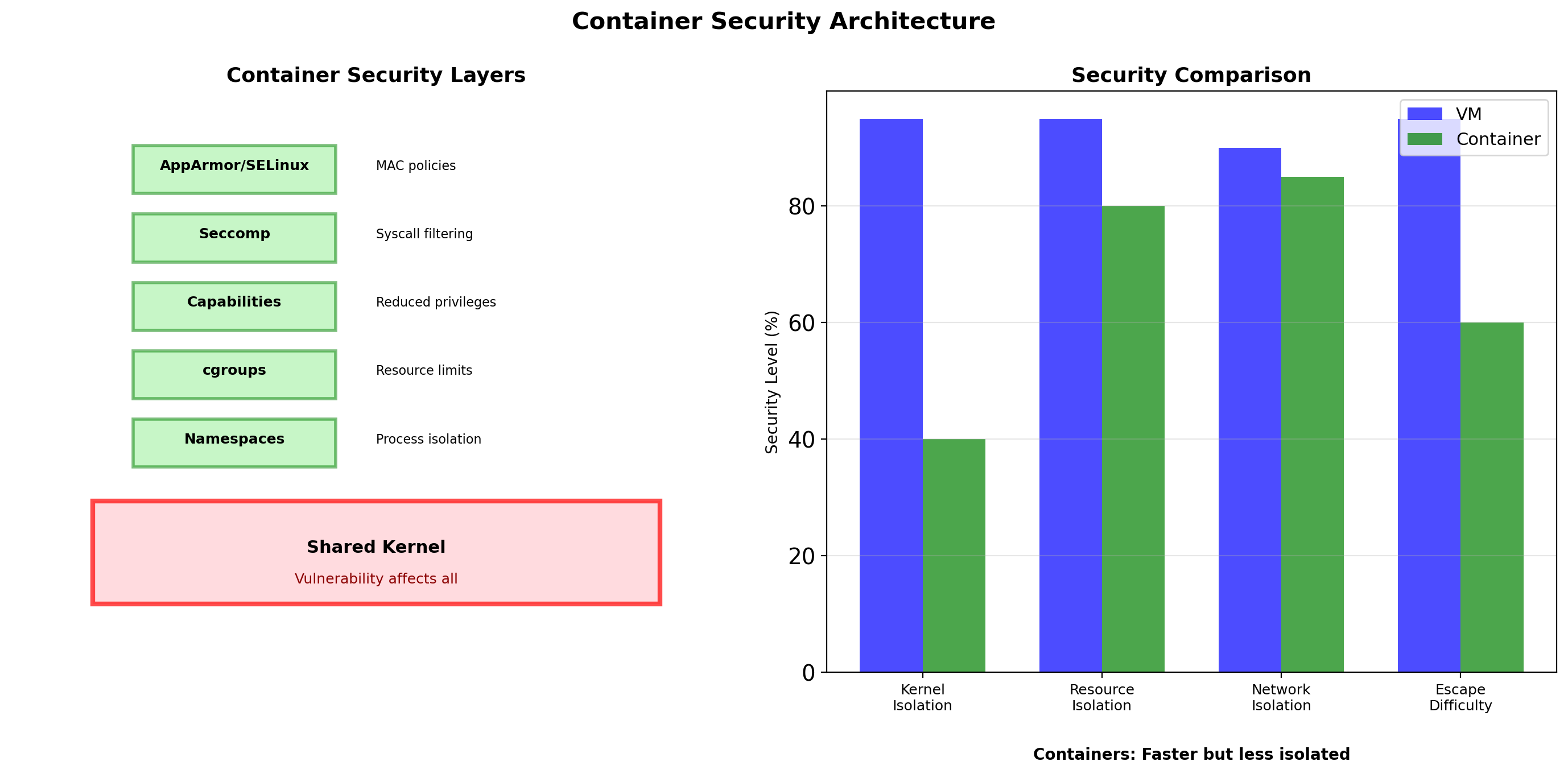
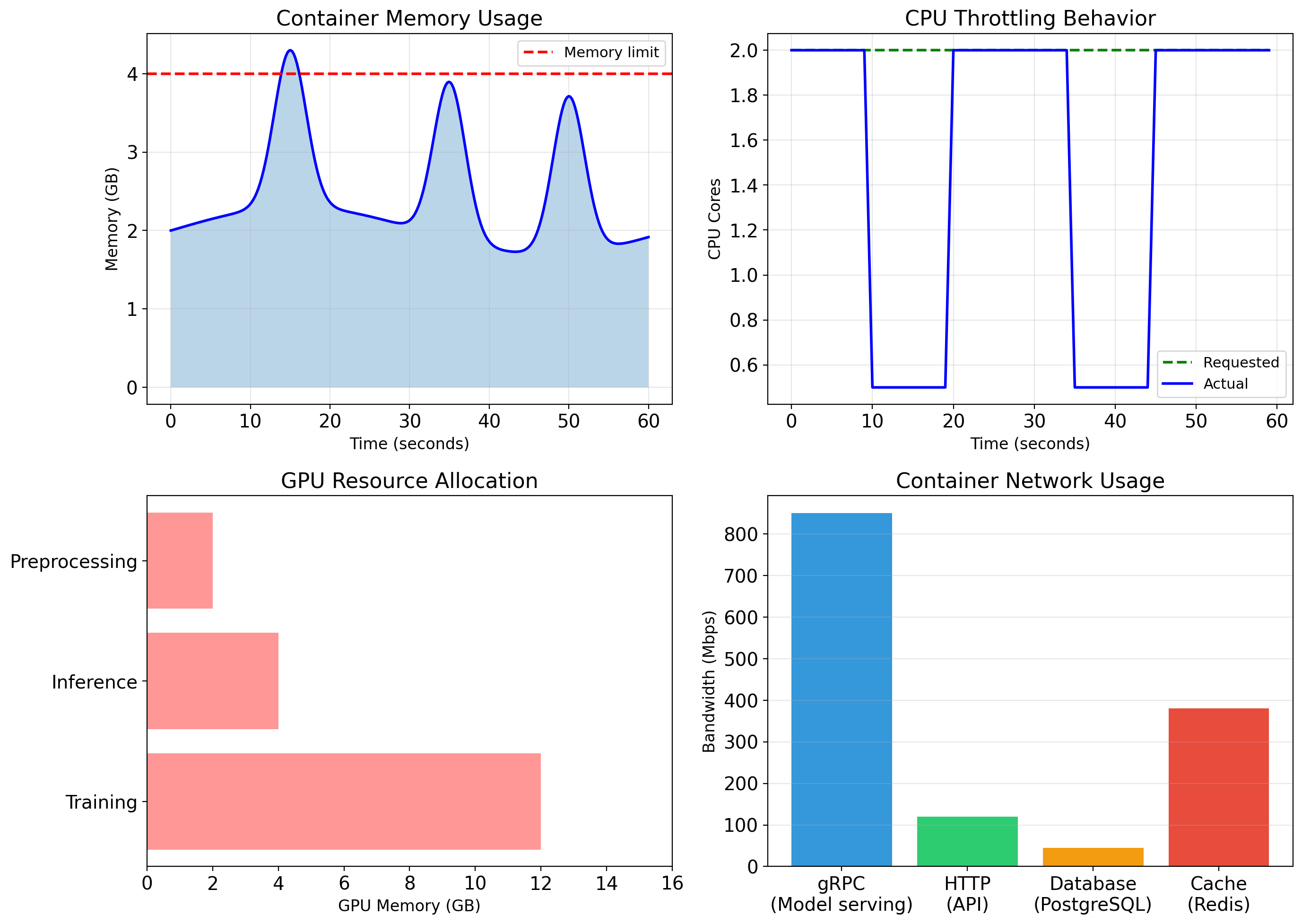
Cgroups Limit Resource Consumption
Namespaces provide isolation—processes can’t see each other. But they don’t prevent resource exhaustion.
Without limits, one container could:
- Consume all available CPU
- Exhaust system memory
- Saturate disk I/O
Control groups (cgroups) let the kernel limit resources per container.
# Container limited to:
# - 2 CPU cores
# - 4 GB memory
# - 100 MB/s disk I/O
If the container exceeds its memory limit, the kernel kills processes inside that container—not processes in other containers or on the host.
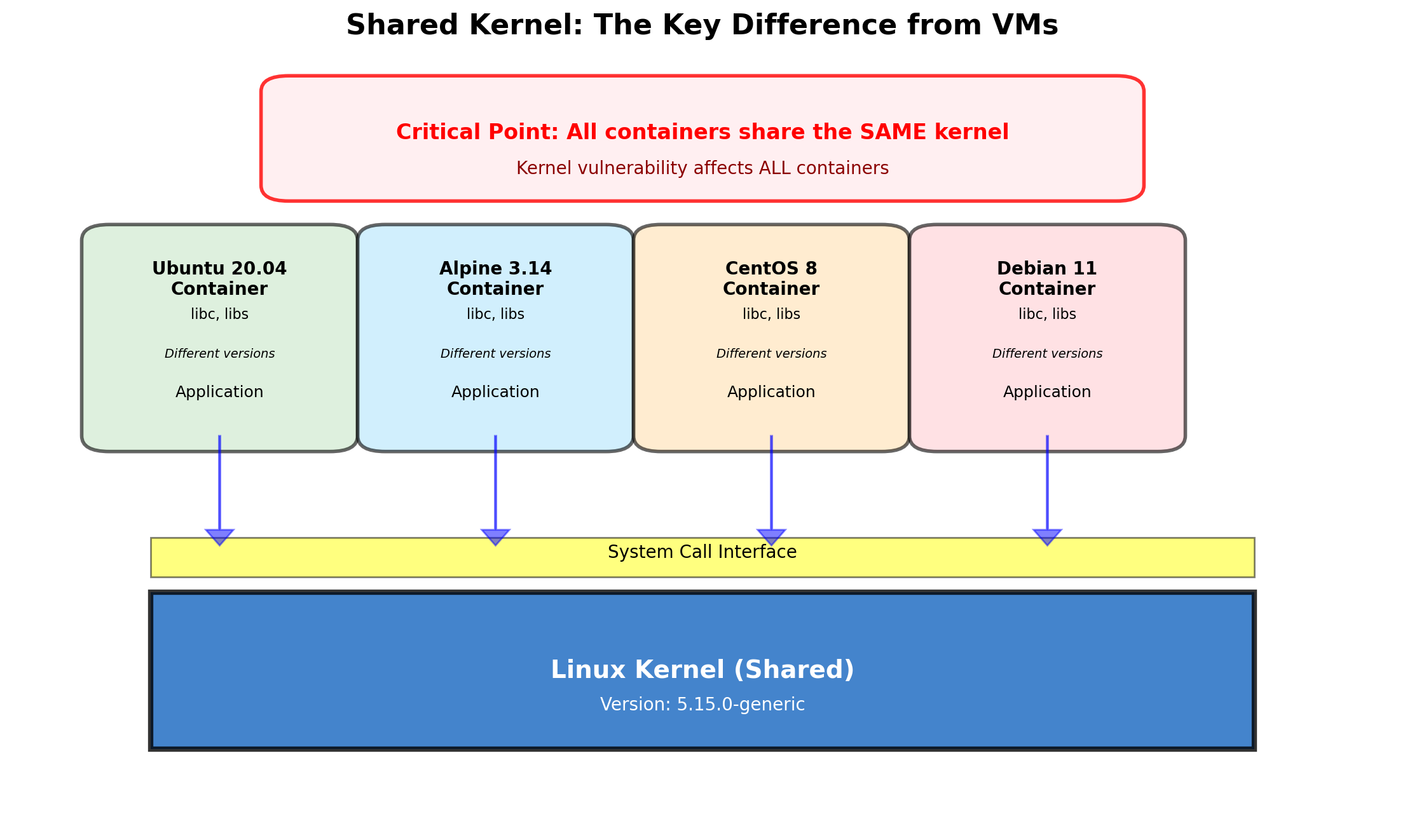
Containers vs VMs: Different Isolation Mechanisms

VMs run separate kernels. Containers share the host kernel.
VMs are isolated by hardware virtualization. Containers are isolated by kernel namespaces.
Container Startup is Fast
VMs boot an operating system: kernel initialization, init system, service startup.
Containers start a process. The kernel is already running. The container runtime sets up namespaces and cgroups, then executes the application.
This speed difference enables different deployment patterns—containers can be started and stopped rapidly in response to demand.
Container Density is High
A server with 256 GB RAM running VMs:
| Component | Memory |
|---|---|
| Hypervisor | ~2 GB |
| Per-VM OS overhead | ~1-2 GB |
| Available for 10 VMs | ~236 GB |
| Per-VM for applications | ~20-23 GB |
Same server running containers:
| Component | Memory |
|---|---|
| Host OS | ~2 GB |
| Container runtime | ~200 MB |
| Available for containers | ~253 GB |
| Per-container overhead | ~10-50 MB |

Namespaces and Cgroups Existed Before Docker
The Linux kernel has provided namespaces since 2002 and cgroups since 2007. Containers were possible—but painful to use.
To create a container manually:
- Create namespace for PID, mount, network, etc.
- Set up a root filesystem
- Configure cgroup limits
- Set up networking (veth pairs, bridges)
- Handle DNS, hostname, users
- Actually run the application
Each step requires detailed knowledge of kernel interfaces. Different tools for each piece. No standard format for packaging.
Docker, released in 2013, made containers accessible. Not by inventing containers—by making them usable.
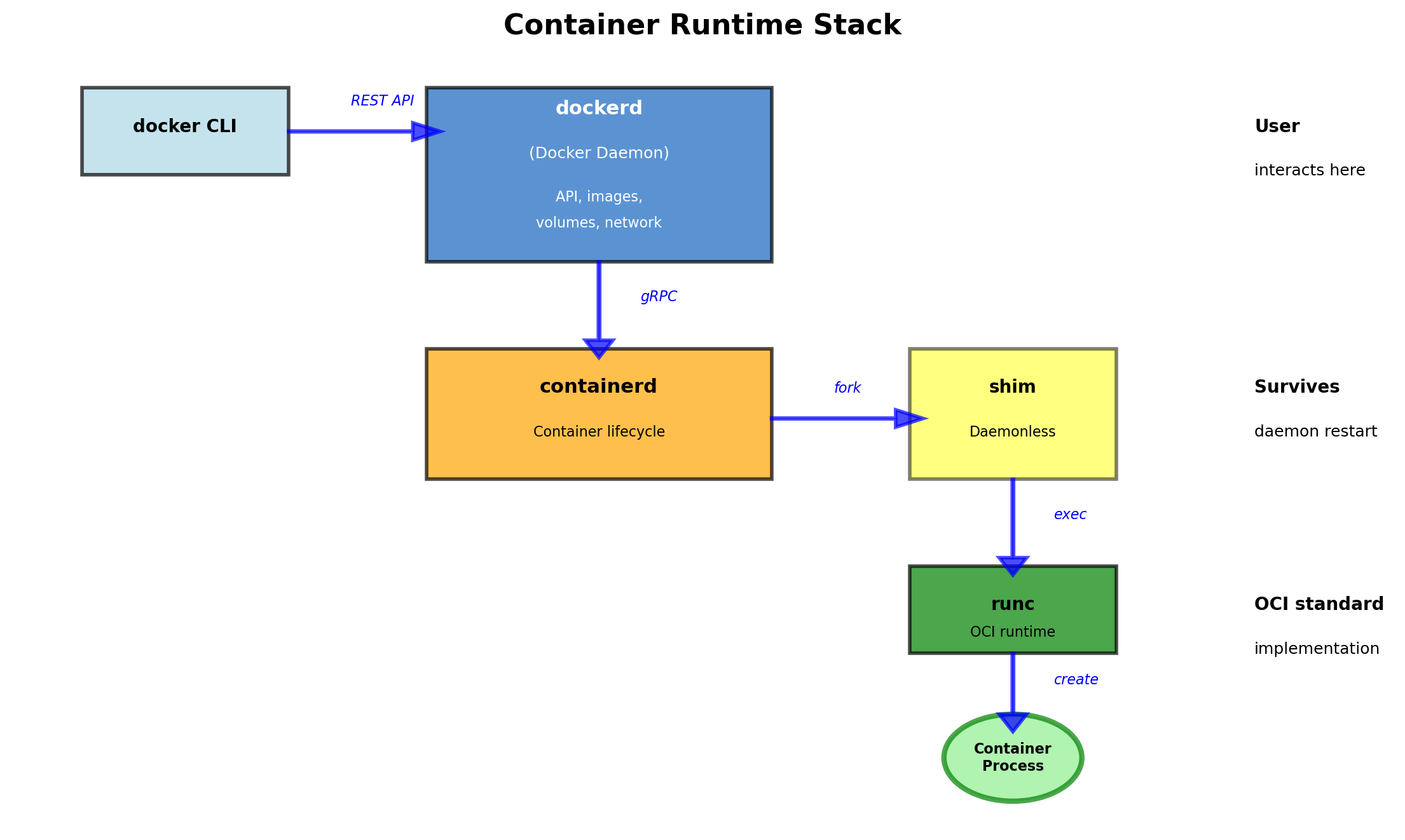
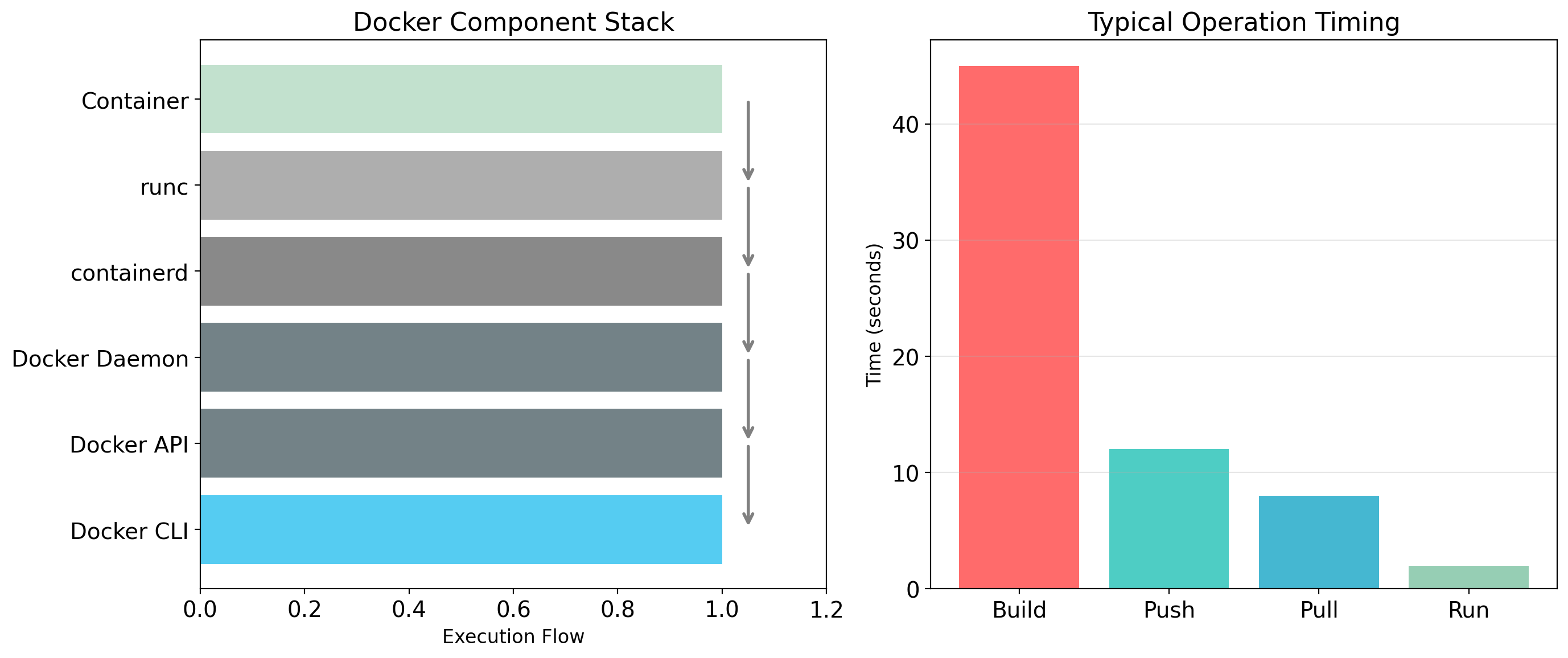
Docker Provides Tooling, Not Technology
Docker is a set of tools that make containers practical:
Image format
A standard way to package an application with its dependencies. Portable across machines running Docker.
Build system
Dockerfiles describe how to create images. Reproducible, automated builds.
Distribution
Registries store and serve images. Push images from one machine, pull to another.
Runtime
Commands to run, stop, inspect containers. Manages namespaces, cgroups, networking behind the scenes.
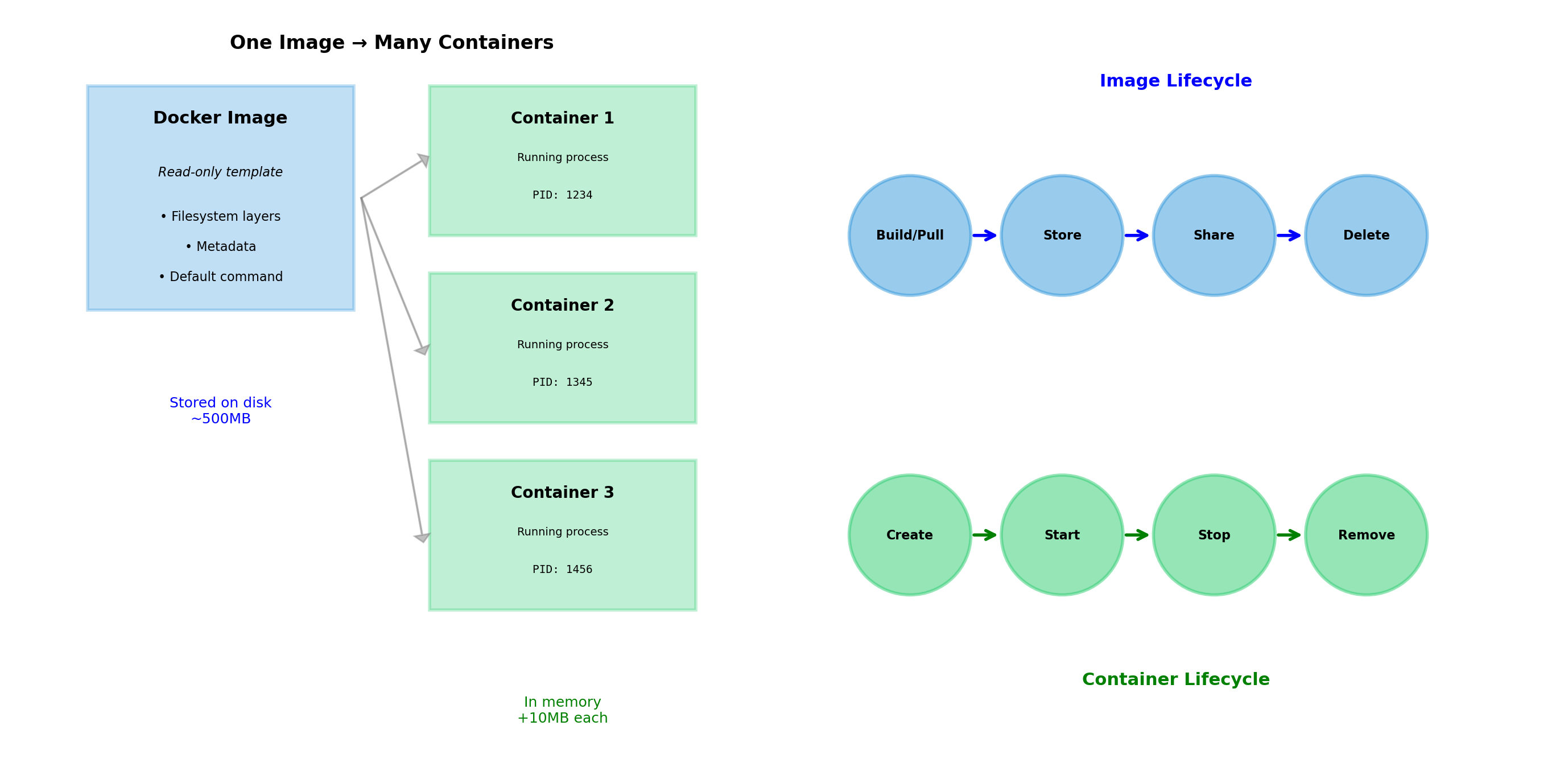
Images and Containers Are Different Things
Image
A read-only template. Contains:
- Filesystem contents (application code, libraries, config)
- Metadata (what command to run, environment variables)
Images are immutable. Once built, they don’t change.
Container
A running instance of an image. Has:
- The image’s filesystem (read-only)
- A writable layer for runtime changes
- Running processes
- Network interfaces
- State (running, stopped, etc.)
Many containers can run from the same image. Each has its own writable layer and process state.
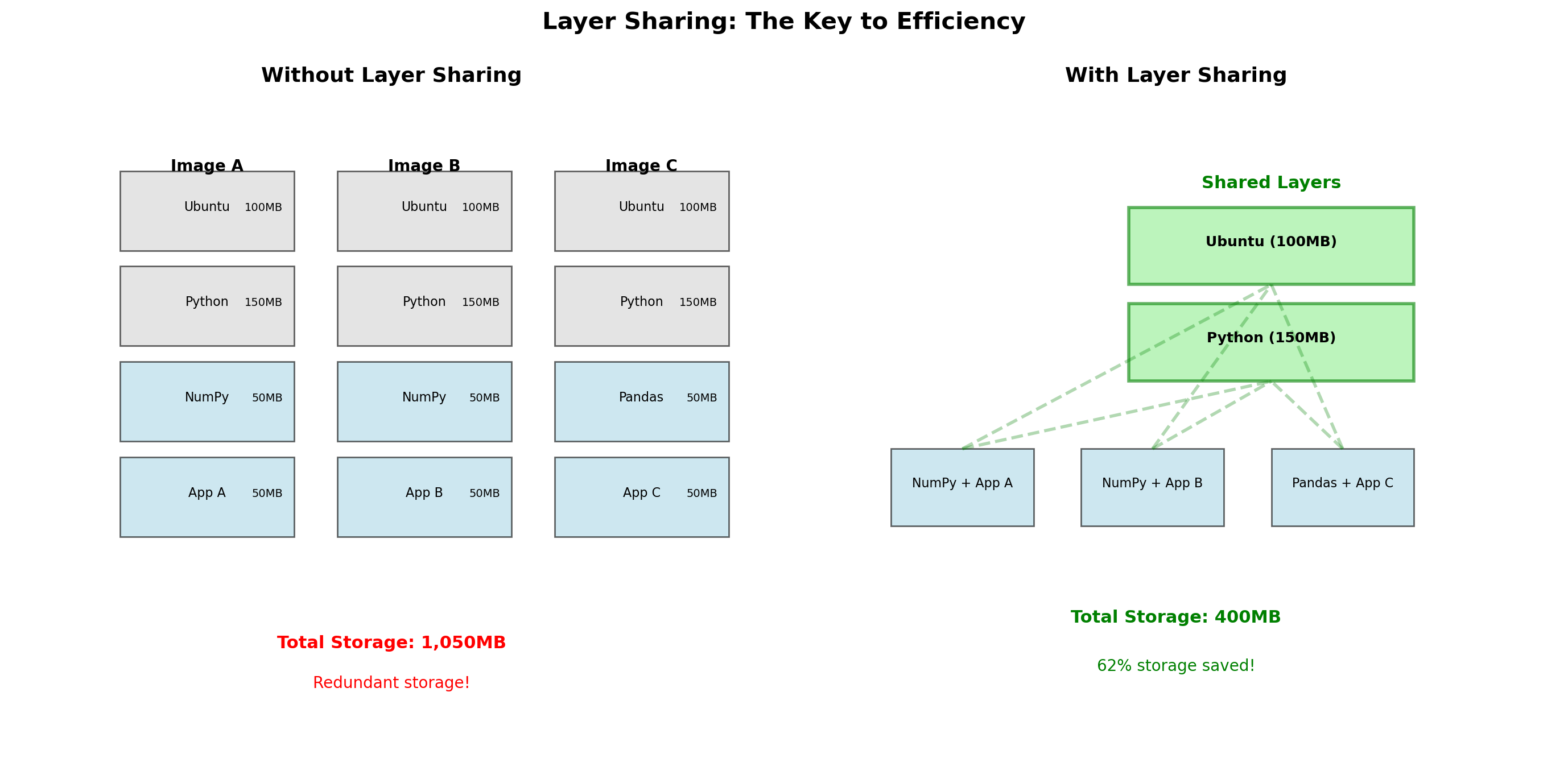
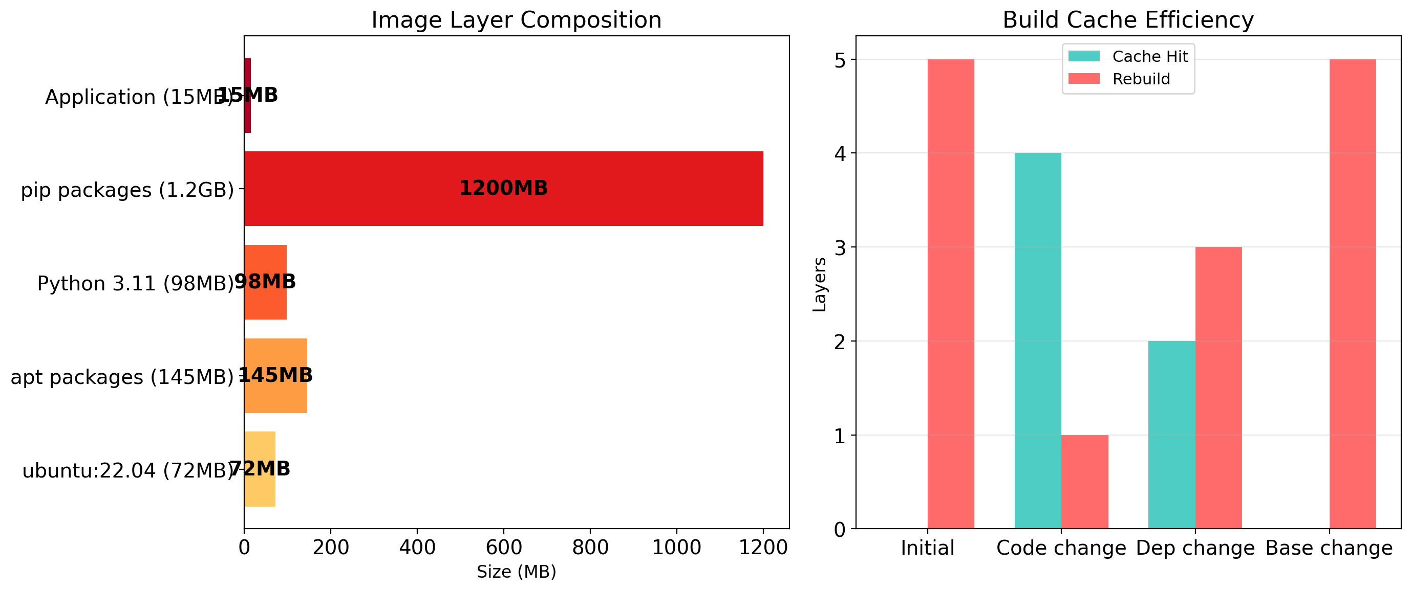
Images Are Built from Layers
An image is not a single blob. It’s a stack of layers.
Each layer represents a change:
- Base layer: Ubuntu filesystem
- Layer 2:
apt install python - Layer 3:
pip install flask - Layer 4: Copy application code
Layers are read-only and content-addressed. If two images share a base layer, they share the actual bytes on disk.
Image A             Image B
┌───────────┐       ┌───────────┐
│ my app    │       │ other app │
├───────────┤       ├───────────┤
│ flask     │       │ django    │
├───────────┼───────┼───────────┤
│        python:3.11          │
├─────────────────────────────┤
│           ubuntu            │
└─────────────────────────────┘
         (shared layers)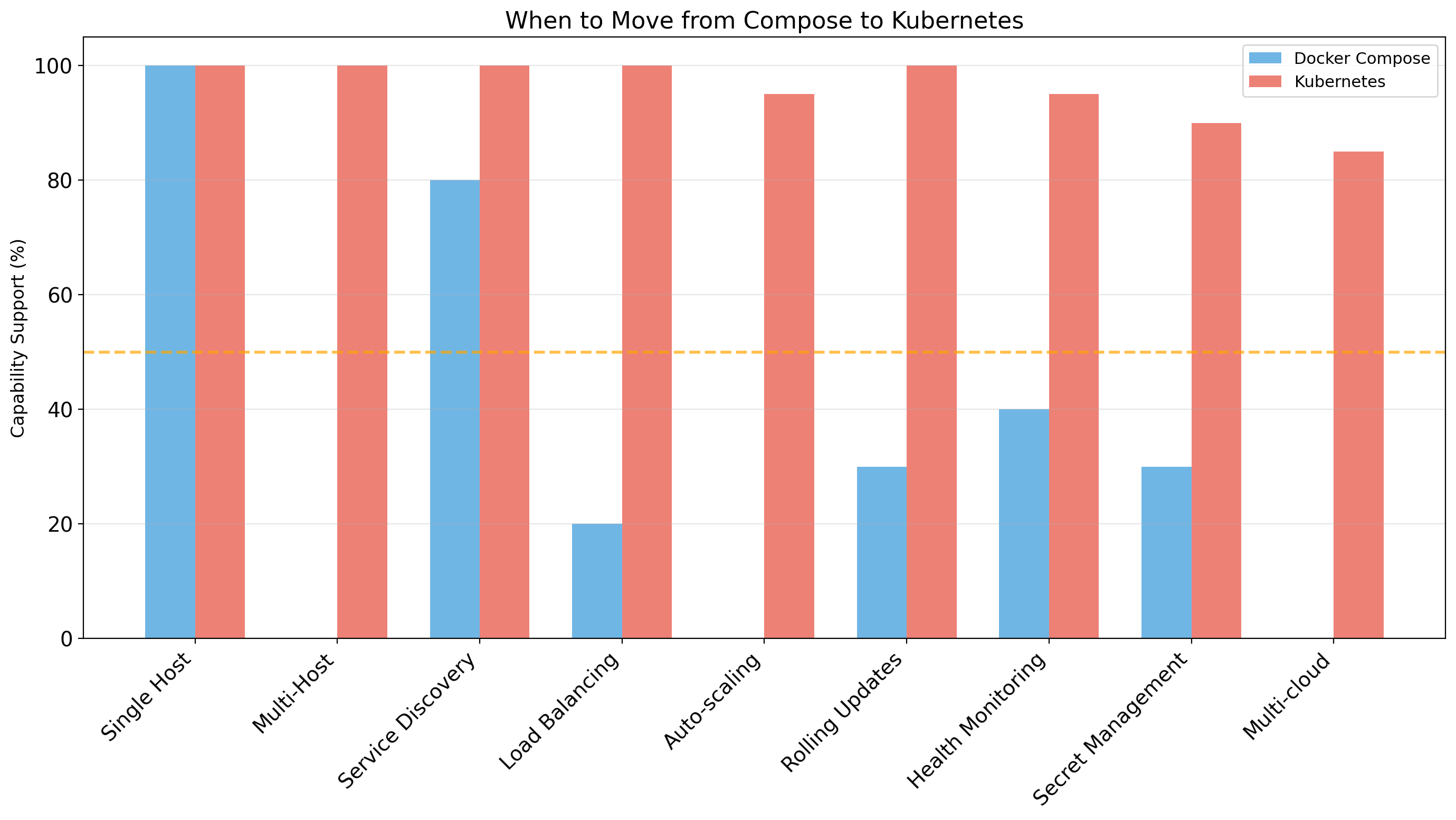
Layer Sharing Saves Space and Time
Storage efficiency
Ten applications using python:3.11 share one copy of that layer. 800 MB base × 10 = 800 MB, not 8 GB.
Distribution efficiency
Pulling a new image version that only changed application code? Only download the changed layer. The base layers are already present.
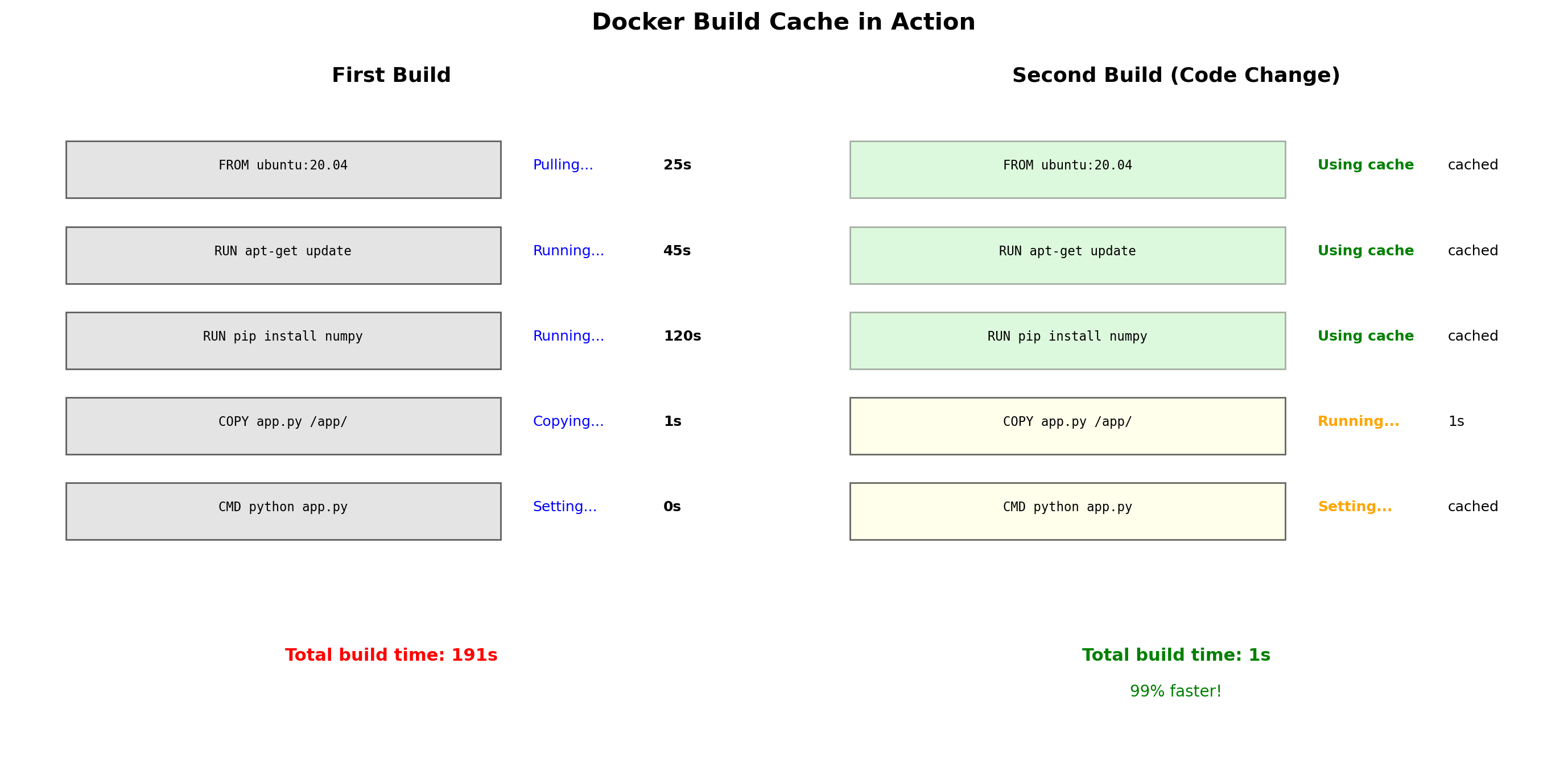
Build efficiency
Rebuilding after a code change? Docker reuses cached layers that haven’t changed. Only the COPY . /app layer needs to rebuild.
Layer ordering matters
Put things that change frequently (application code) in later layers. Put things that change rarely (OS, dependencies) in earlier layers.
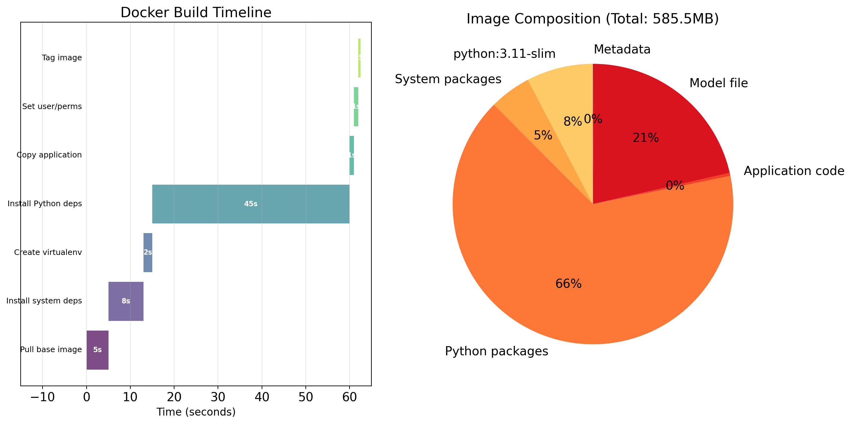
Building an Image
$ docker build -t myapp:v1 .The build process:
- Docker reads the Dockerfile
- Creates a temporary container from the base image
- Executes each instruction in that container
- Saves the result as a new layer
- Stacks layers into the final image
The build context
The . specifies the build context—the directory whose contents are available to COPY commands. Docker sends this to the daemon before building.
Large build contexts slow down builds. Use .dockerignore to exclude unnecessary files.
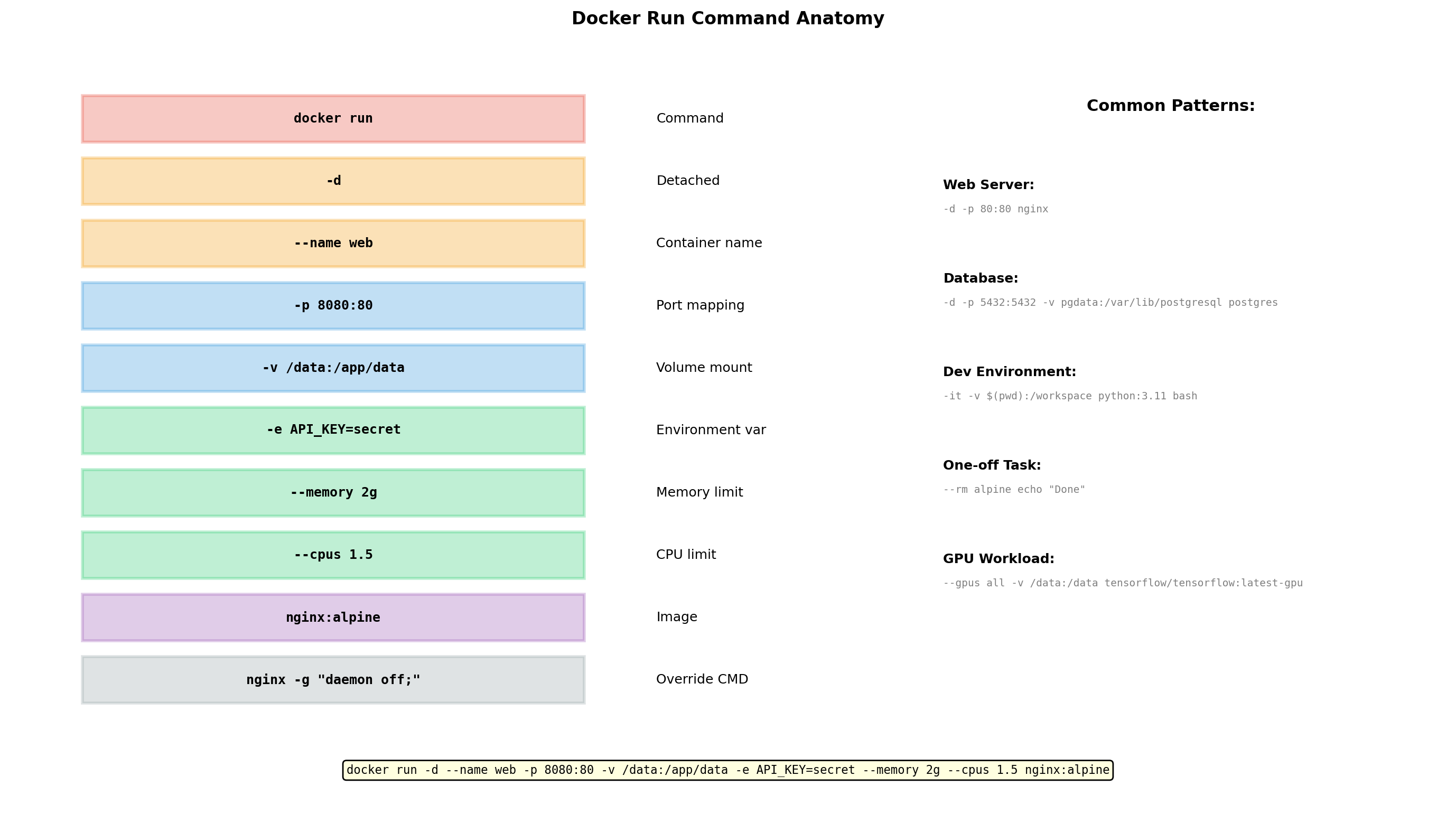
Running a Container
$ docker run myapp:v1Docker:
- Creates container from image
- Sets up namespaces (PID, mount, network, etc.)
- Creates writable layer on top of image layers
- Configures cgroups if limits specified
- Executes the
CMDorENTRYPOINT
Foreground vs detached
# Foreground - attached to terminal
$ docker run myapp:v1

# Detached - runs in background
$ docker run -d myapp:v1
Naming containers
$ docker run --name my-api myapp:v1Without --name, Docker assigns a random name.
Port Mapping Connects Containers to the Network
Containers have isolated network namespaces. A container listening on port 8080 is not accessible from the host by default.
Port mapping connects host ports to container ports:
$ docker run -p 8080:80 nginxThis means: traffic to host port 8080 goes to container port 80.
Host                        Container
┌──────────┐    -p 8080:80   ┌──────────┐
│ :8080    │ ──────────────> │ :80      │
└──────────┘                 └──────────┘
Multiple mappings
$ docker run -p 8080:80 -p 8443:443 nginx
Container Filesystems Are Ephemeral
Changes to a container’s filesystem are stored in its writable layer. When the container is removed, that layer is deleted.
$ docker run -d --name mydb postgres
$ docker exec mydb psql -c "CREATE TABLE users..."
# Database file created in container's writable layer

$ docker rm -f mydb
# Container removed - data gone

$ docker run -d --name mydb postgres
# Fresh container - no users table
This is a feature, not a bug. Containers are disposable. Same image always starts from the same state.
But databases, uploaded files, and logs need to persist beyond container lifetime.
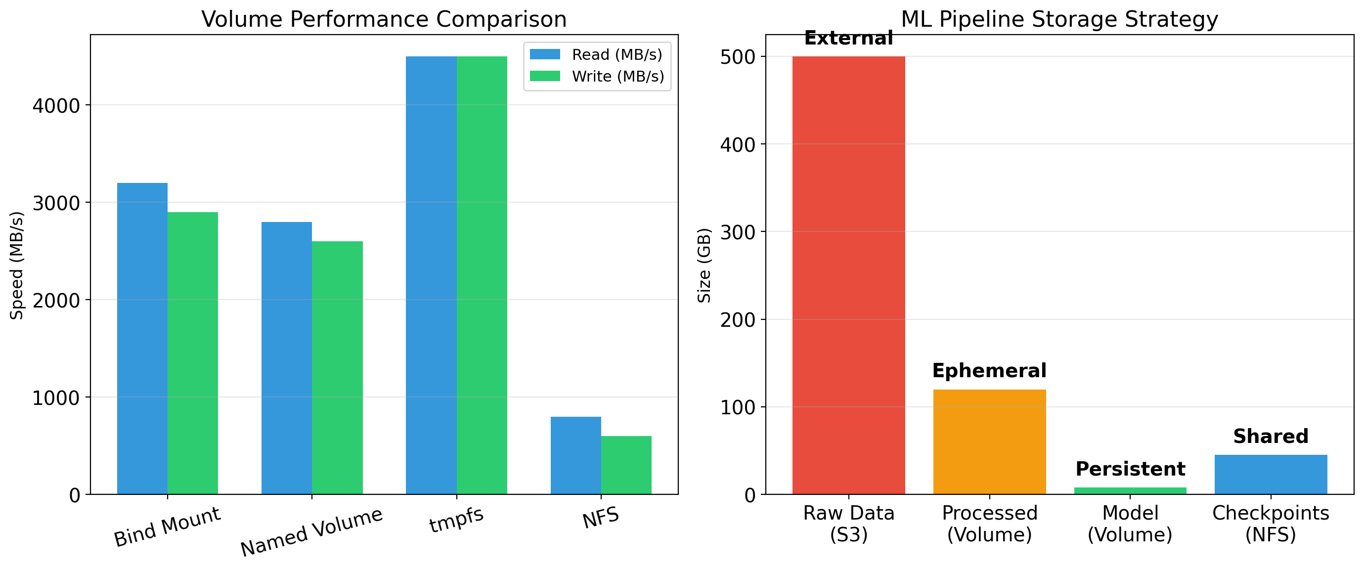
Volumes Persist Data Beyond Container Lifetime
A volume is storage managed by Docker that exists outside the container’s filesystem.
# Named volume
$ docker run -v pgdata:/var/lib/postgresql/data postgres
The volume pgdata persists even when the container is removed. A new container can attach to the same volume.
$ docker rm -f mydb
$ docker run -v pgdata:/var/lib/postgresql/data postgres
# Same data, new container
Bind mounts map a host directory into the container:
$ docker run -v /host/path:/container/path myappUseful for development—edit code on host, container sees changes.
Environment Variables Configure Containers
Many applications are configured through environment variables. Docker makes this easy:
$ docker run -e DATABASE_URL=postgres://db:5432 \
             -e API_KEY=secret123 \
             myapp
Inside the container, the application reads these:
import os
db_url = os.environ['DATABASE_URL']
api_key = os.environ['API_KEY']
Why environment variables?
- Same image, different configuration per environment
- Secrets don’t need to be baked into images
- Twelve-factor app pattern
Multiple variables
$ docker run -e VAR1=value1 -e VAR2=value2 myapp
Container Networking: Containers Communicate
Containers on the same Docker network can communicate using container names.
# Create a network
$ docker network create mynet

# Run database on that network
$ docker run -d --name db --network mynet postgres

# Run app on same network
$ docker run -d --name api --network mynet \
    -e DATABASE_URL=postgres://db:5432/app \
    myapp
The api container connects to db by name. Docker provides DNS resolution within the network.
No port mapping needed for container-to-container traffic. Port mapping is only for external access.

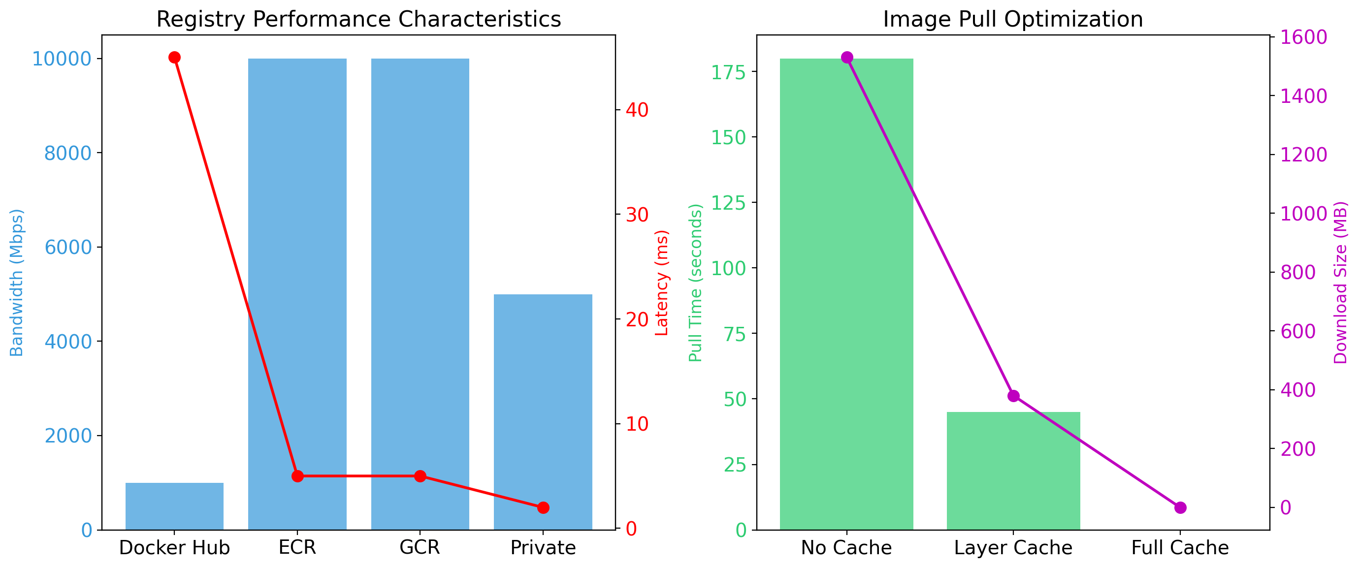
Registries Store and Distribute Images
Images need to move between machines—from build server to production, from developer to teammate.
Docker Hub is the default public registry. Millions of images available.
$ docker pull nginx        # From Docker Hub
$ docker pull python:3.11  # Specific version
Private registries for proprietary images:
- Amazon ECR
- Google Container Registry
- Azure Container Registry
- Self-hosted registry
$ docker login my-registry.example.com
$ docker push my-registry.example.com/myapp:v1
Image naming
registry/repository:tag
gcr.io/my-project/myapp:v1.2.3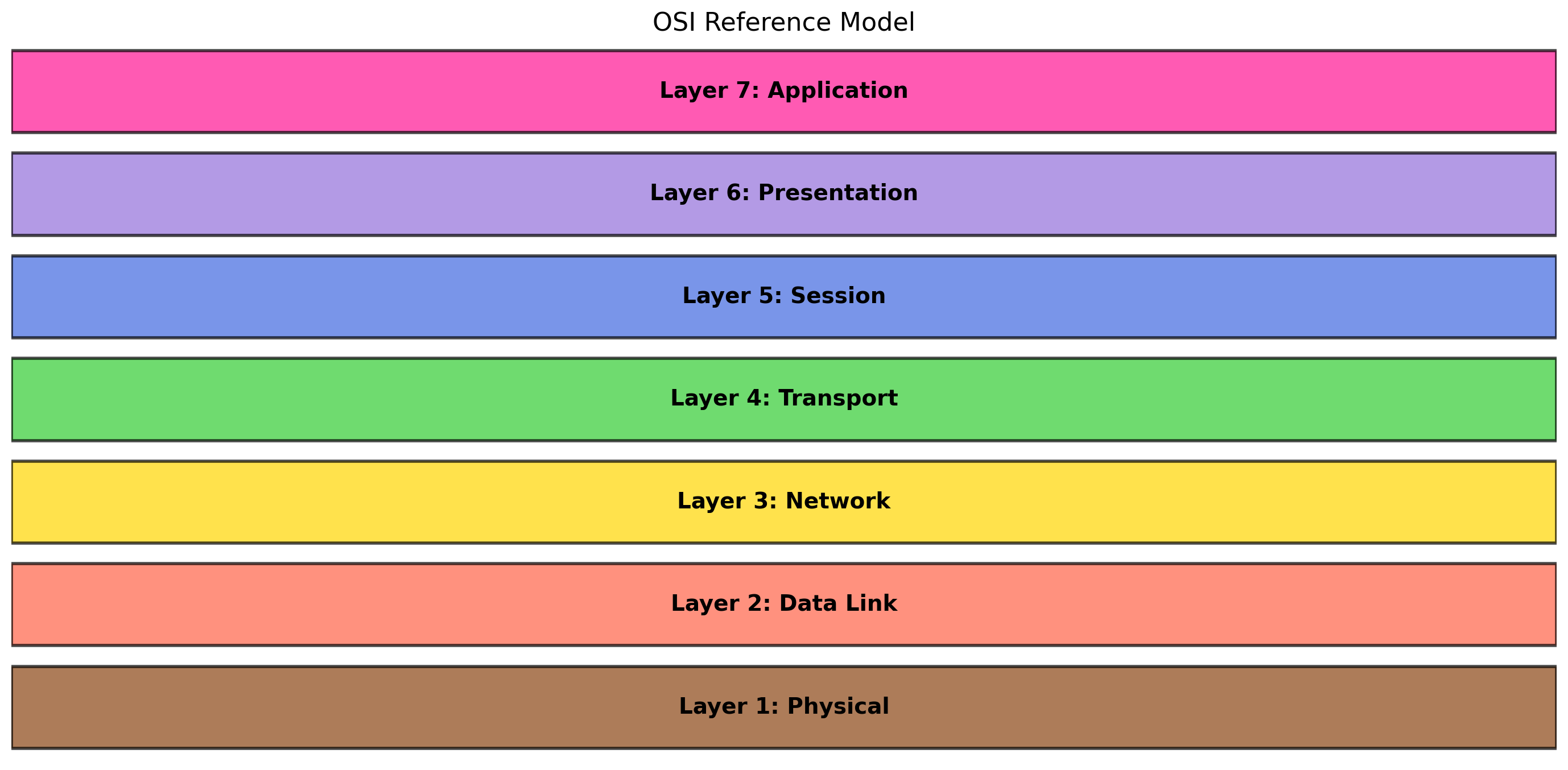
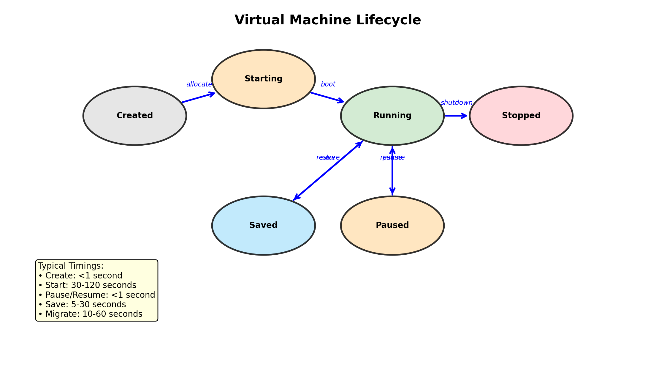
Container Lifecycle
Containers have states:
# Create and start
$ docker run -d --name web nginx
# State: running

# Stop (graceful shutdown)
$ docker stop web
# State: stopped (exited)

# Start again
$ docker start web
# State: running

# Remove
$ docker rm web
# Container deleted

# Force remove running container
$ docker rm -f web
Listing containers
$ docker ps          # Running containers
$ docker ps -a       # All containers (including stopped)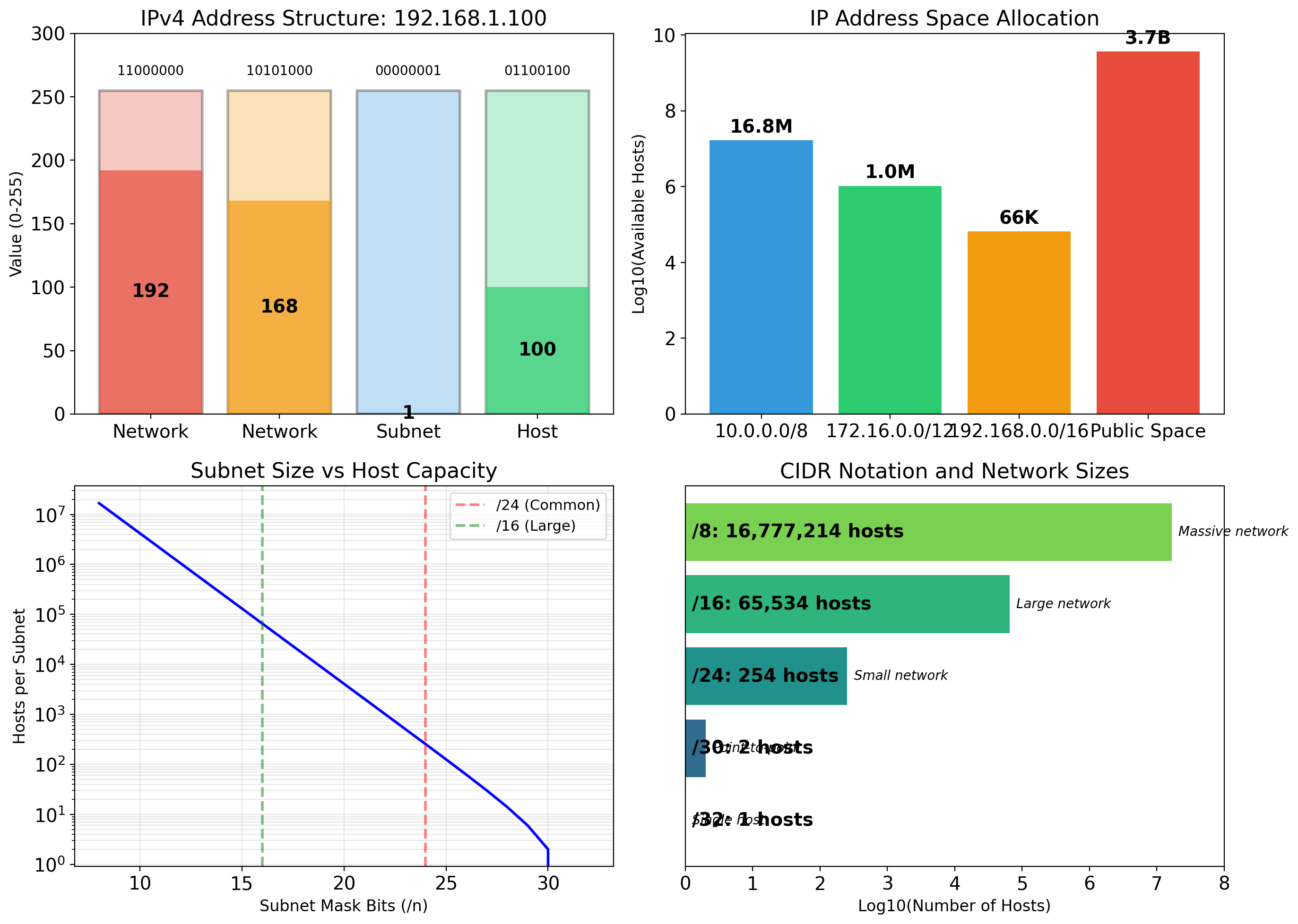
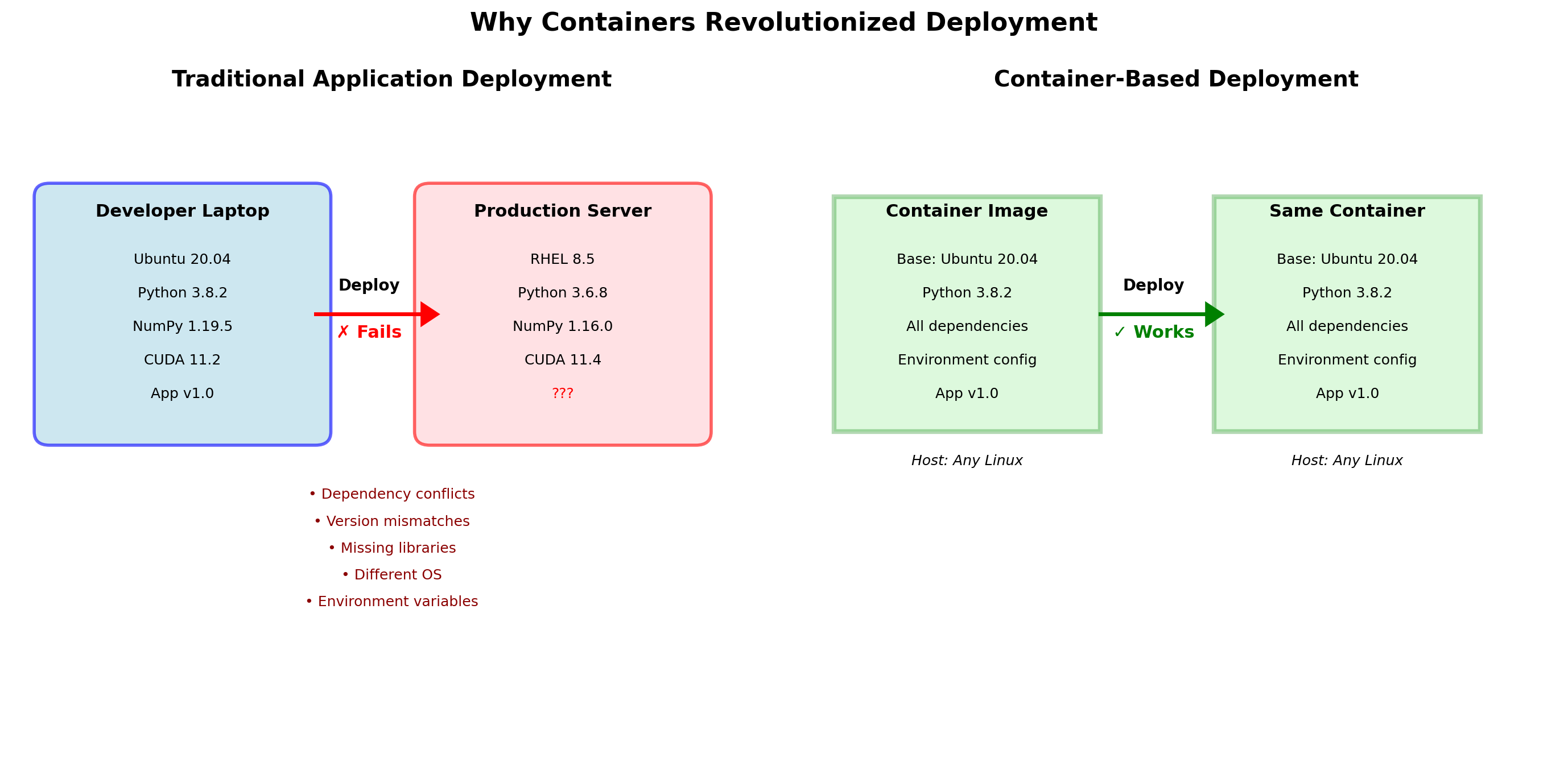
Docker Enables Reproducible Environments
The “works on my machine” problem
- Developer has Python 3.11, server has Python 3.9
- Developer has OpenSSL 3.0, server has 1.1.1
- Developer’s PATH includes local tools
Docker’s solution
The image contains everything the application needs. The same image runs the same way on:
- Developer laptop
- CI/CD server
- Staging environment
- Production
Build the image once. Test it. Deploy the same image to production. No environment drift.
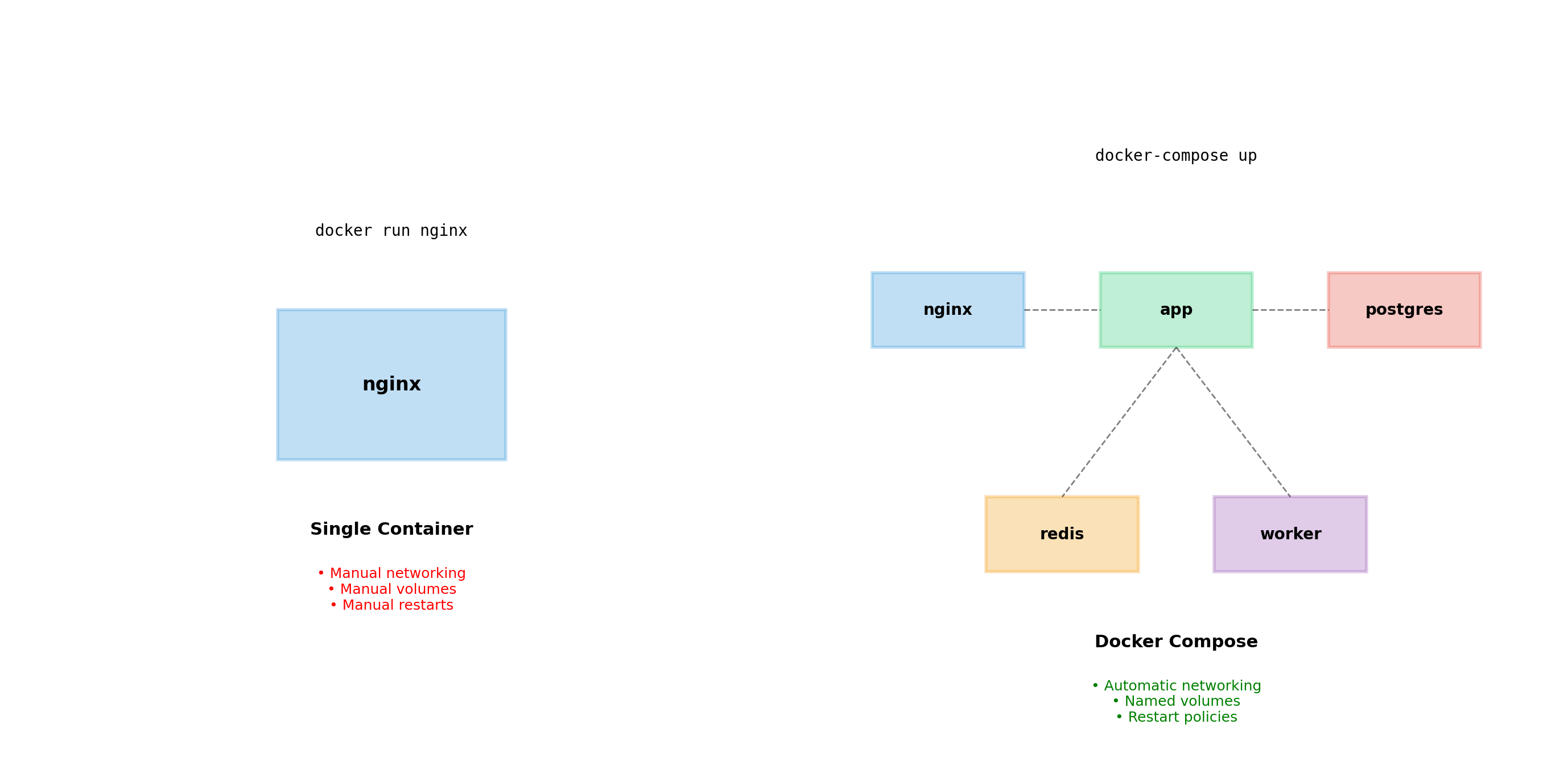
Real Applications Have Multiple Containers
A web application typically requires several services:
- Web server — handles HTTP, serves static files
- Application server — runs business logic
- Database — stores persistent data
- Cache — speeds up frequent queries
- Background worker — processes async jobs
Each service runs in its own container. They need to communicate, share data, and start in the right order.
With what we’ve covered so far, this means many docker run commands with careful coordination.

depends_on Controls Start Order, Not Readiness
A common misconception: depends_on waits for the dependency to be “ready.”
What actually happens:
api:
  depends_on:
    - db
Compose starts db first, then starts api immediately after.
It does not wait for:
- PostgreSQL to finish initializing
- The database to accept connections
- Any health check to pass
The problem:
Database containers often take several seconds to initialize. Your API container starts, tries to connect, and fails because the database isn’t ready yet.

Compose Creates a Default Network
When you run docker compose up, Compose automatically:
- Creates a network named
{project}_default - Connects all services to this network
- Sets up DNS so services can reach each other by name
services:
  api:
    environment:
      DATABASE_URL: postgres://db:5432/app
      #                       ^^
      # Service name becomes hostname
The api container can connect to db:5432. Docker’s internal DNS resolves db to the database container’s IP address.
No need to know IP addresses. No need to create networks manually. Service names are stable identifiers.
Development Workflow with Compose
Compose is particularly valuable for local development.
Mount source code for live reload:
services:
  api:
    build: ./api
    volumes:
      - ./api:/app  # Mount local code into container
    environment:
      FLASK_DEBUG: "1"  # Enable auto-reload
Edit code on your machine. The container sees changes immediately. Flask (or your framework’s dev server) reloads automatically.
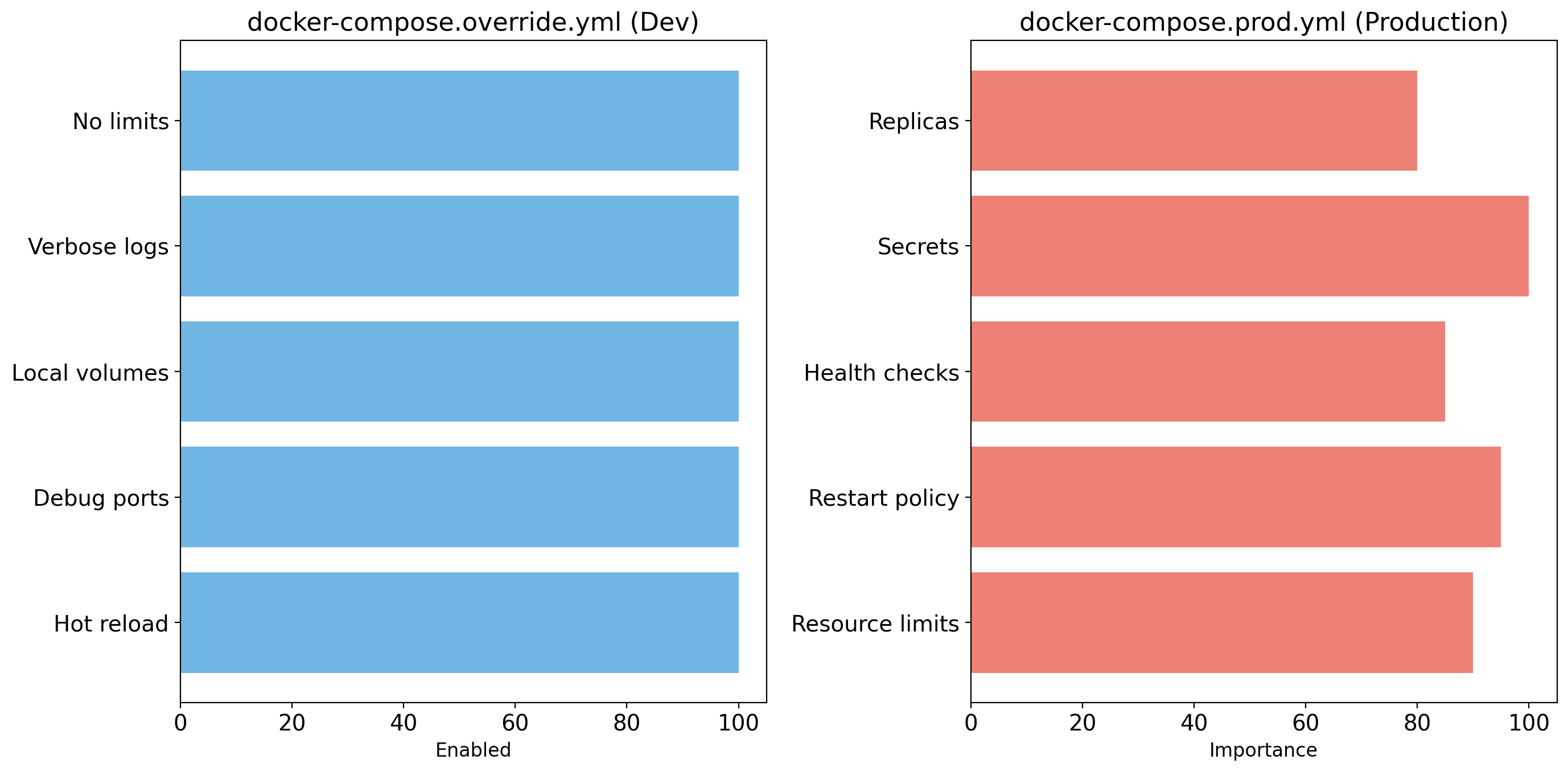
Override files for dev vs prod:
# docker-compose.yaml - base configuration
# docker-compose.override.yaml - dev overrides (auto-loaded)
# docker-compose.prod.yaml - production settings

# Development (uses override automatically)
docker compose up

# Production
docker compose -f docker-compose.yaml -f docker-compose.prod.yaml up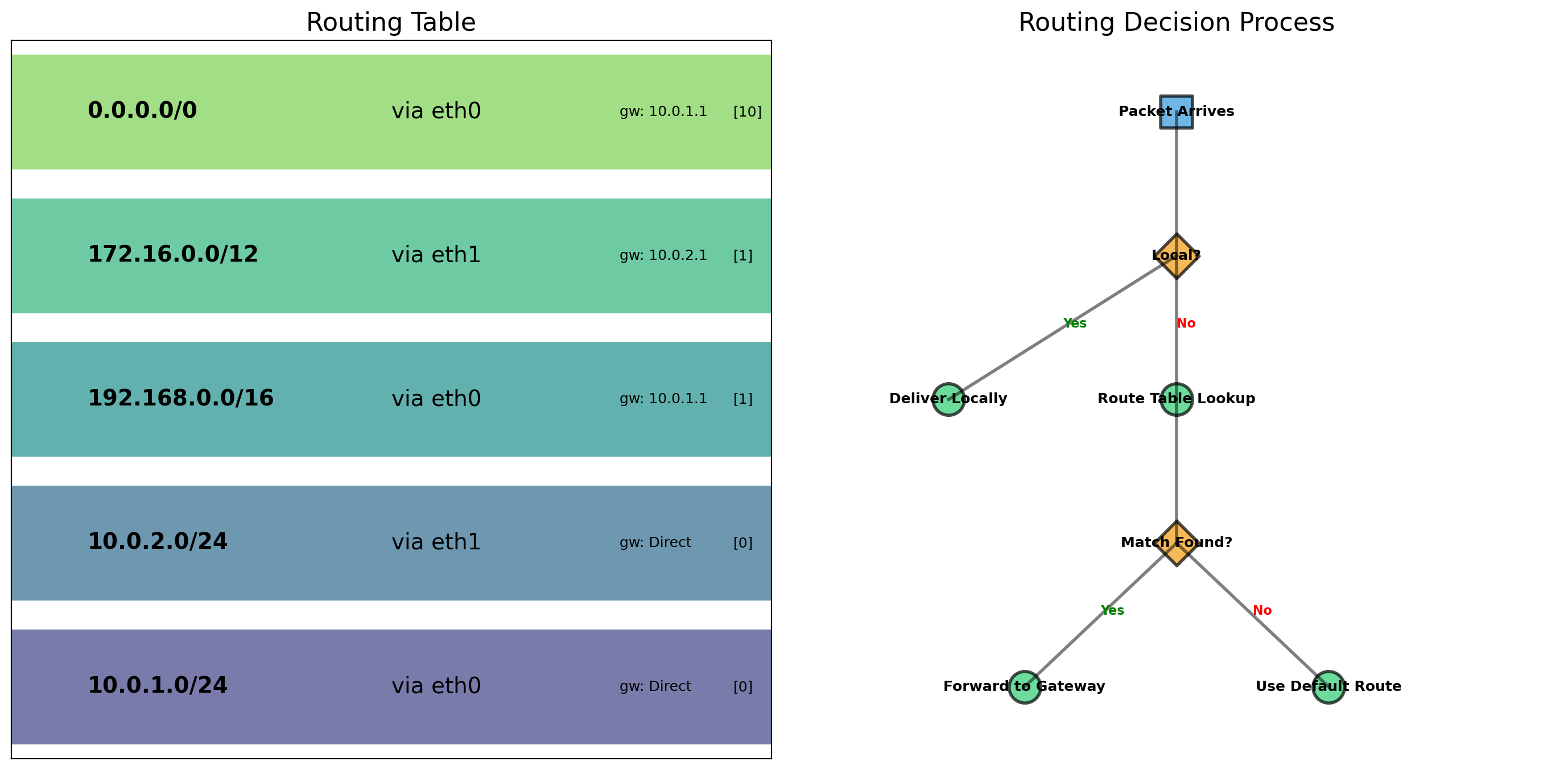
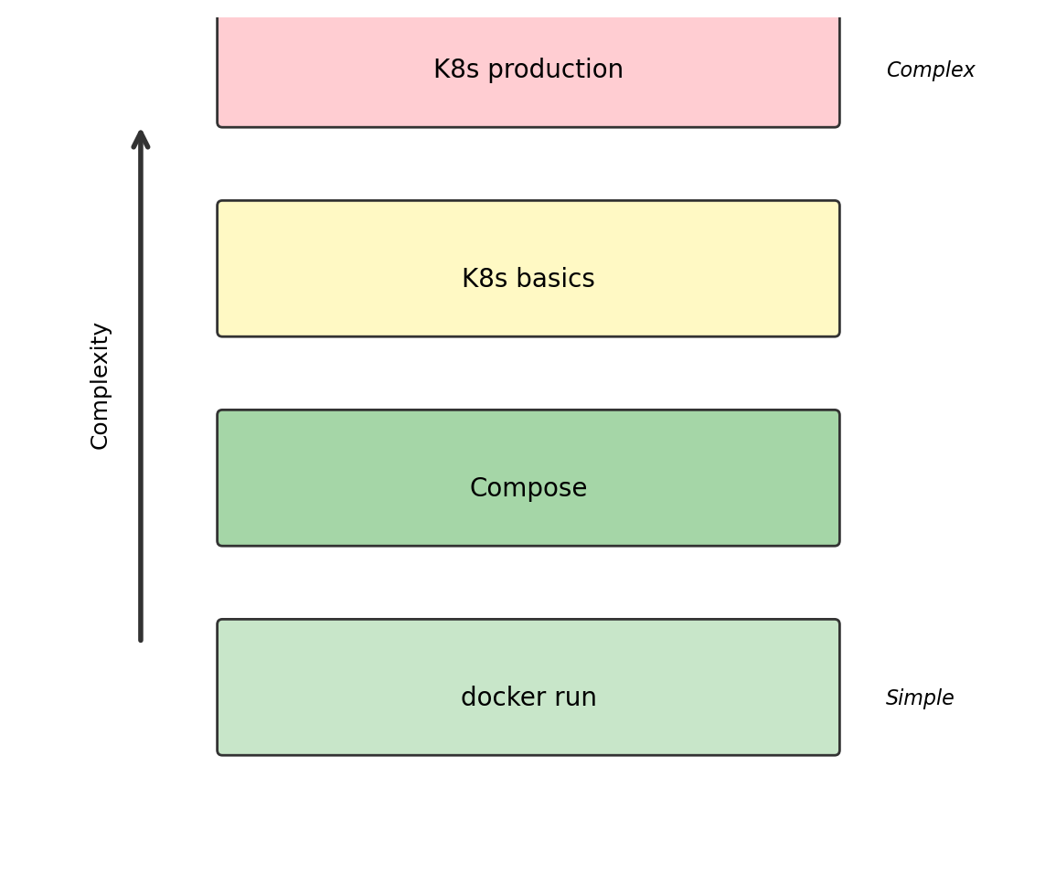
Compose vs Kubernetes: Different Tools, Different Scale
Compose is often sufficient. Don’t add Kubernetes complexity until you need its capabilities.
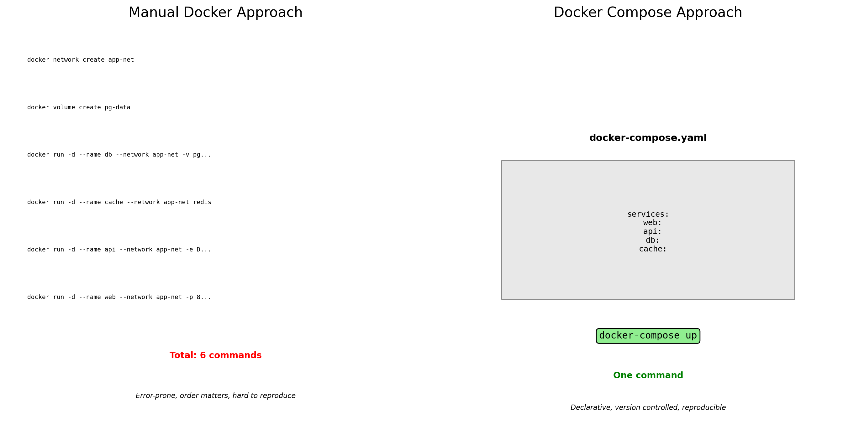
Docker Compose Manages Containers on One Host
Compose solves multi-container coordination on a single machine:
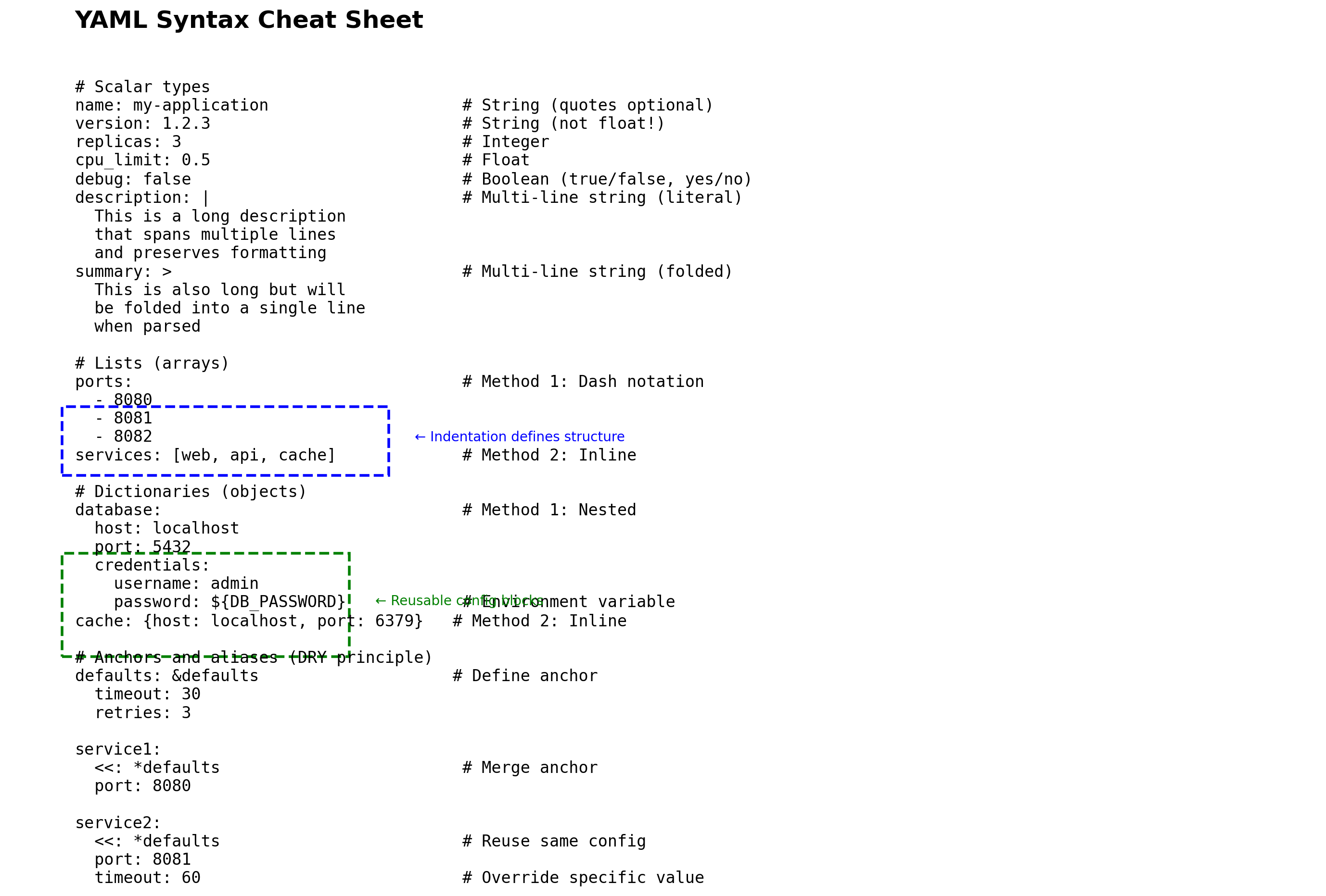
- Define services in YAML
- Bring up entire application with one command
- Containers communicate by service name
- Shared volumes for data persistence
This works well for:
- Local development
- CI/CD testing
- Small-scale deployments
But the application runs on one machine. That machine is a single point of failure.
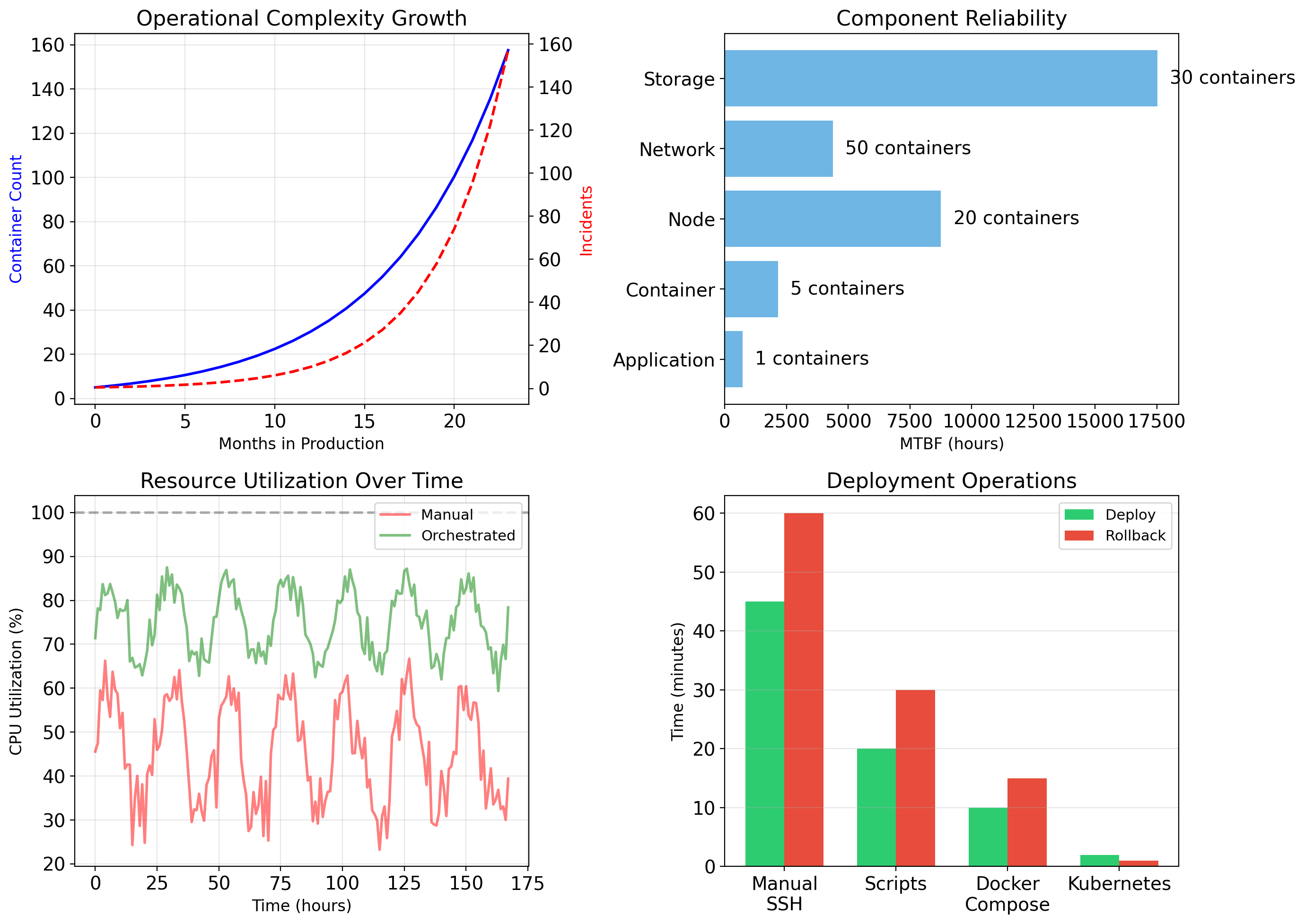
Multi-Host Deployment Requires Coordination
Running containers across multiple machines introduces new problems:
Scheduling
Which container runs on which machine? Need to consider available resources, existing workloads, constraints.
Networking
Containers on different hosts need to communicate. Container on Host A needs to reach container on Host B.
Service discovery
IP addresses change when containers restart or move. How do services find each other?
Failure recovery
Container crashes or host fails. Who notices? Who restarts the container? On which host?
Rolling updates
Deploying new version without downtime. Gradually replace old containers with new ones.
Container Orchestration Systems
Orchestration systems manage containers across clusters of machines.
They handle:
- Scheduling: Deciding where containers run
- Scaling: Running more or fewer instances based on demand
- Networking: Connecting containers across hosts
- Self-healing: Detecting and recovering from failures
- Rolling updates: Deploying new versions without downtime
- Configuration: Injecting settings and secrets
Major orchestration systems:
- Kubernetes — The dominant platform, originally from Google
- Docker Swarm — Docker’s built-in orchestration (simpler, less adopted)
- Amazon ECS — AWS-specific container service
- Nomad — HashiCorp’s alternative

Kubernetes Dominates Container Orchestration
Kubernetes (K8s) emerged from Google’s internal container system (Borg). Open-sourced in 2014, now maintained by the Cloud Native Computing Foundation.
Why Kubernetes won:
- Open source with broad industry support
- Runs on any infrastructure (cloud, on-premise, hybrid)
- Extensive ecosystem of tools and extensions
- All major cloud providers offer managed Kubernetes
Market reality:
Most organizations running containers at scale use Kubernetes. Job postings for “DevOps” or “Platform Engineer” typically require Kubernetes experience.
Understanding Kubernetes concepts—even without operating clusters—is valuable background for working in modern infrastructure.
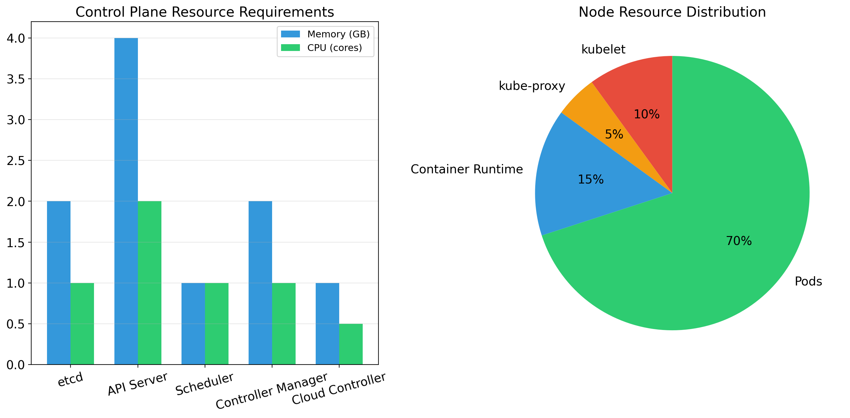
Kubernetes Cluster Architecture
A Kubernetes cluster has two types of machines:
Control Plane (master nodes)
The “brain” of the cluster. Runs:
- API Server: All operations go through REST API
- Scheduler: Decides which node runs each workload
- Controller Manager: Maintains desired state
- etcd: Distributed database storing cluster state
Worker Nodes
The machines that run your containers:
- Kubelet: Agent that manages containers on the node
- Container Runtime: Actually runs containers (containerd, CRI-O)
- Kube-proxy: Handles networking for services
Pods: The Smallest Deployable Unit
Kubernetes does not manage containers directly. It manages Pods.
A Pod is:
- One or more containers that share resources
- The atomic unit of scheduling
- What Kubernetes creates, destroys, and moves
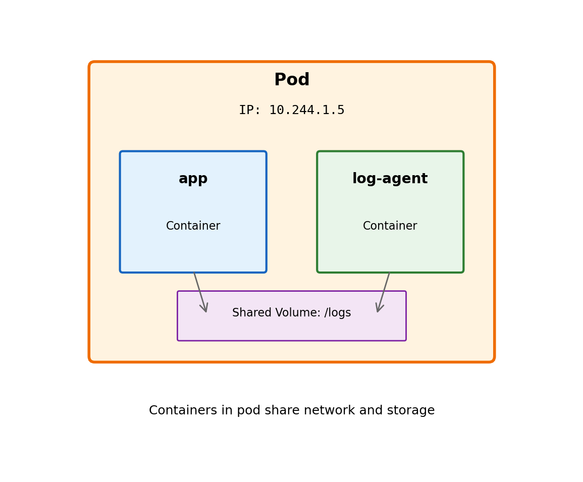
Containers in a Pod share:
- Network namespace (same IP address, localhost communication)
- Storage volumes
- Lifecycle (scheduled together, start/stop together)
Why not just containers?
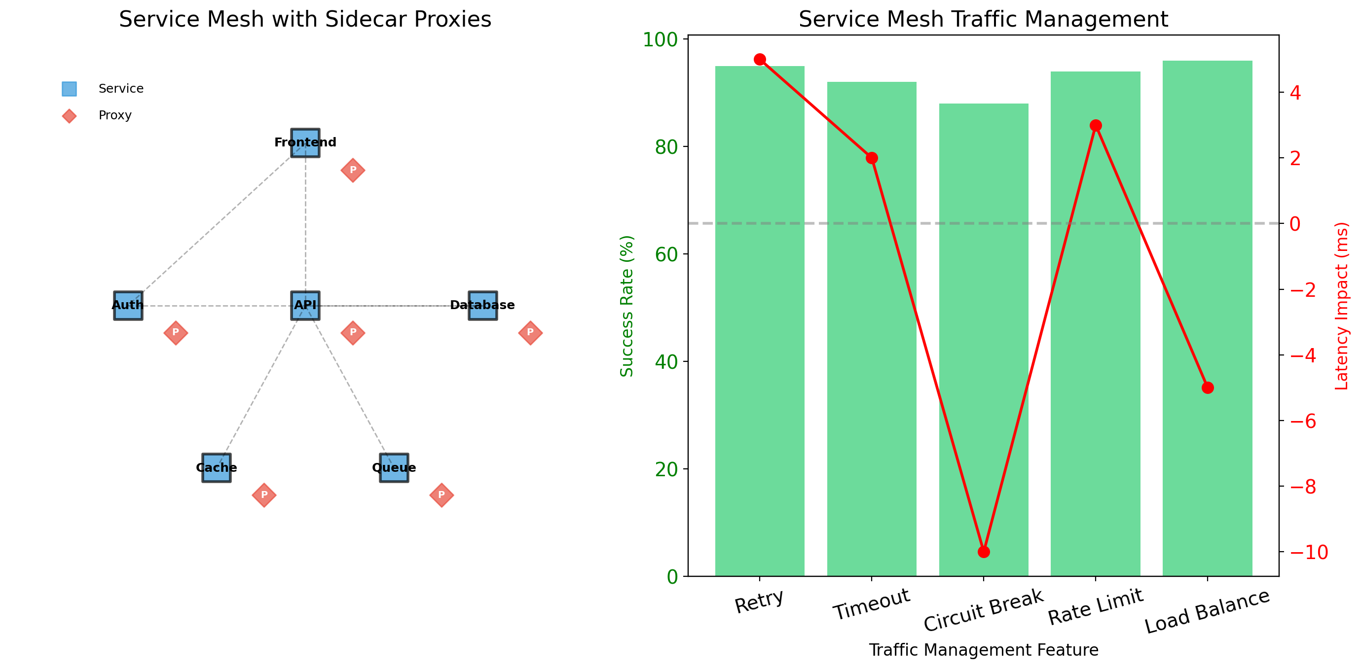
Sometimes tightly-coupled containers need to be co-located. A logging sidecar that reads another container’s files. A proxy that handles network traffic for the main application.
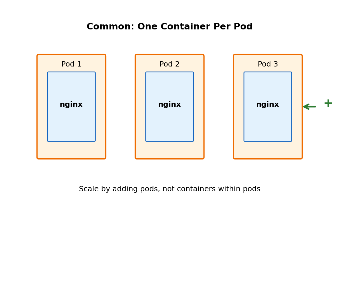
Most Pods Have One Container
Multi-container pods exist for specific patterns:
- Sidecar: Helper container (logging, monitoring, proxy)
- Ambassador: Proxy that simplifies network communication
- Adapter: Transform output format of main container
But the common case is one container per pod.
apiVersion: v1
kind: Pod
metadata:
  name: web-server
spec:
  containers:
  - name: nginx
    image: nginx:1.24
    ports:
    - containerPort: 80
The pod is the management unit. Kubernetes schedules the pod, not the container. When you scale up, you add pods—each containing its container.
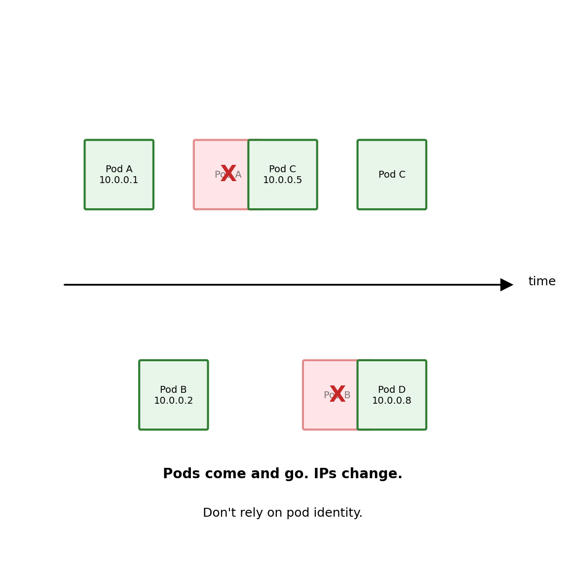
Pods Are Ephemeral
Pods are not permanent. They can be:
- Killed by the scheduler to free resources
- Evicted when a node runs out of memory
- Lost when a node fails
- Replaced during rolling updates
Each new pod gets a new IP address. You cannot rely on a pod’s identity persisting.
This is different from traditional servers where applications run on stable machines with fixed IPs.
Implication:
Don’t connect to pods directly by IP. Don’t store important data only in a pod’s filesystem. Treat pods as disposable.
Kubernetes provides abstractions (Services, Deployments) that handle this ephemerality.
Deployments Manage Pod Lifecycles
You rarely create pods directly. Instead, you create a Deployment.
A Deployment declares:
- What container image to run
- How many replicas (pod instances)
- Resource requirements
- Update strategy
Kubernetes ensures reality matches the declaration:
- Pod crashes → Deployment creates a replacement
- Node fails → Pods rescheduled to other nodes
- You request 5 replicas → Kubernetes maintains exactly 5
apiVersion: apps/v1
kind: Deployment
metadata:
  name: web-server
spec:
  replicas: 3
  template:
    spec:
      containers:
      - name: nginx
        image: nginx:1.24
Deployments Handle Rolling Updates
When you update a Deployment (new image version), Kubernetes performs a rolling update:
- Create one new pod with new version
- Wait until it’s healthy
- Terminate one old pod
- Repeat until all pods are new version
No downtime
Some pods always running during the update. Traffic continues flowing.
Automatic rollback
If new pods fail health checks, Kubernetes stops the rollout. Old pods remain running.
# Update image version
$ kubectl set image deployment/web-server \
    nginx=nginx:1.25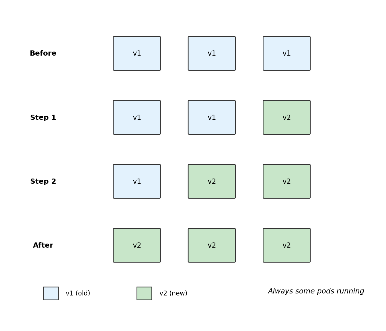
Services Provide Stable Network Endpoints
Pods have ephemeral IP addresses. A Service provides a stable endpoint.
A Service:
- Has a fixed cluster IP address
- Has a DNS name (e.g.,
web-server.default.svc.cluster.local) - Load balances traffic across matching pods
- Tracks pods using label selectors
When a pod dies and is replaced, the Service automatically routes to the new pod. Clients connect to the Service, not individual pods.
apiVersion: v1
kind: Service
metadata:
  name: web-server
spec:
  selector:
    app: web-server
  ports:
  - port: 80
    targetPort: 8080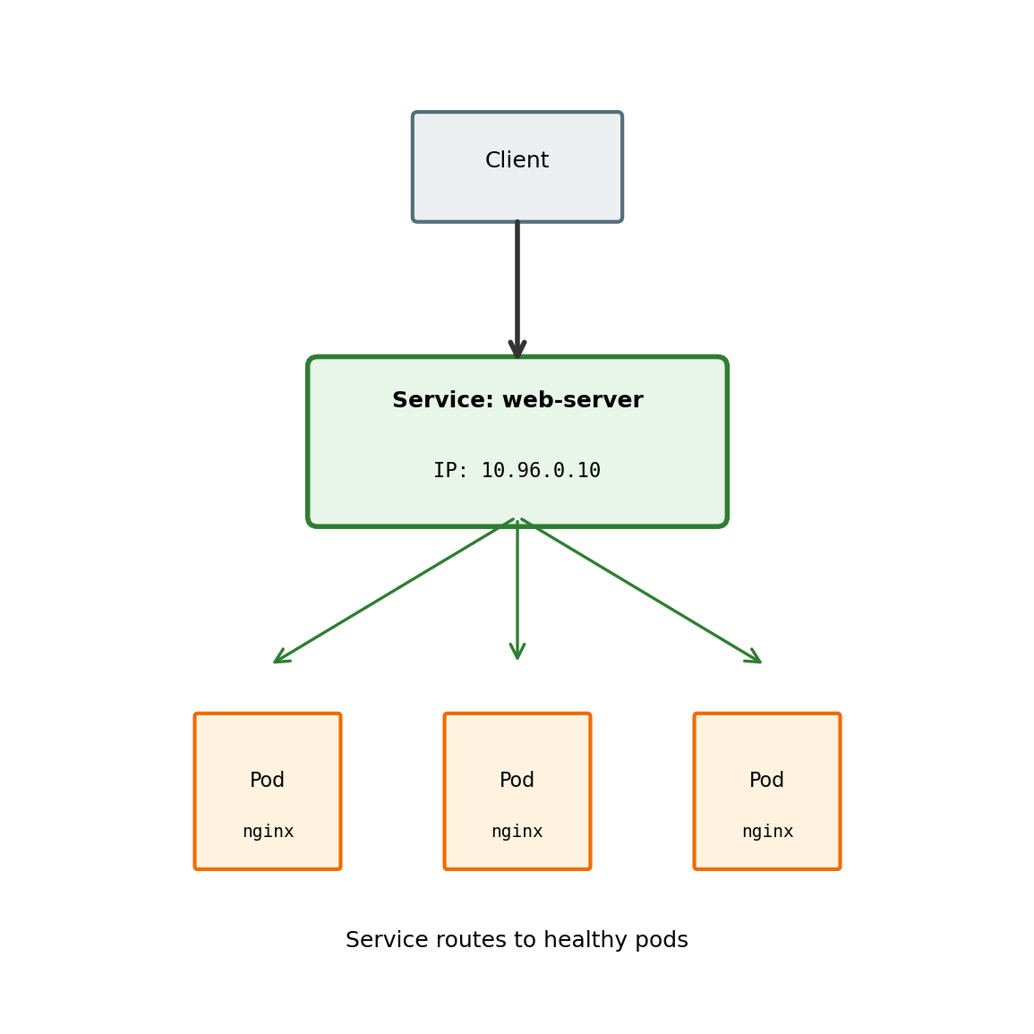
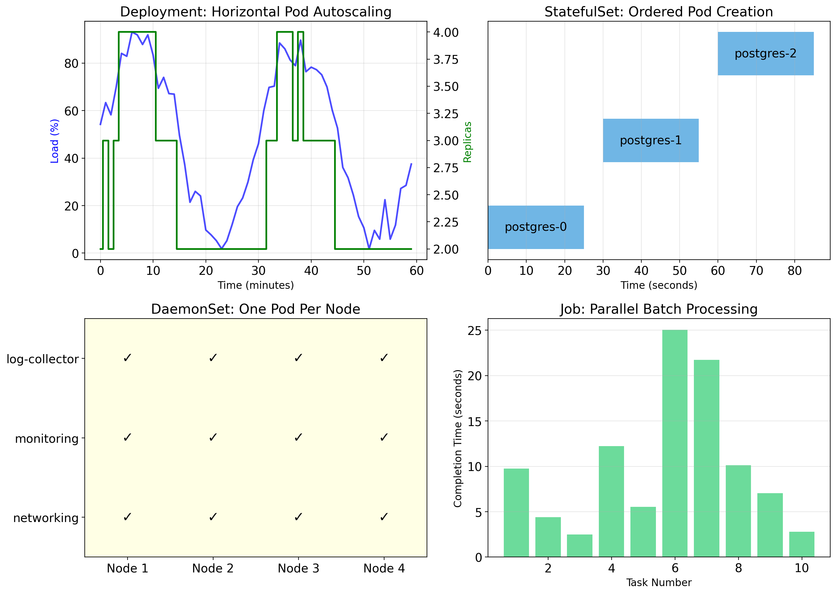
Kubernetes is Complex
The concepts covered here are foundational. Production Kubernetes involves much more:
- Ingress: HTTP routing, TLS termination
- NetworkPolicies: Firewall rules between pods
- PersistentVolumes: Storage management
- StatefulSets: For databases and stateful apps
- DaemonSets: One pod per node (logging, monitoring)
- RBAC: Access control
- Operators: Custom controllers
- Service mesh: Istio, Linkerd for advanced networking
Operating Kubernetes clusters requires significant expertise. Most organizations use managed services (EKS, GKE, AKS) to reduce operational burden.