Every application maintains state while running. A web server tracks active connections. An application server holds session data, cached computations, in-flight request context.
This state exists only in process memory.
Python dictionaries, object attributes, class instances — all reside in the process heap
A running container writes temporary files to its writable layer
Redis holds its dataset in RAM
Application logs accumulate in local buffers
When the process exits, the memory is reclaimed
When the container restarts, the writable layer is replaced
When the instance terminates, local storage is gone
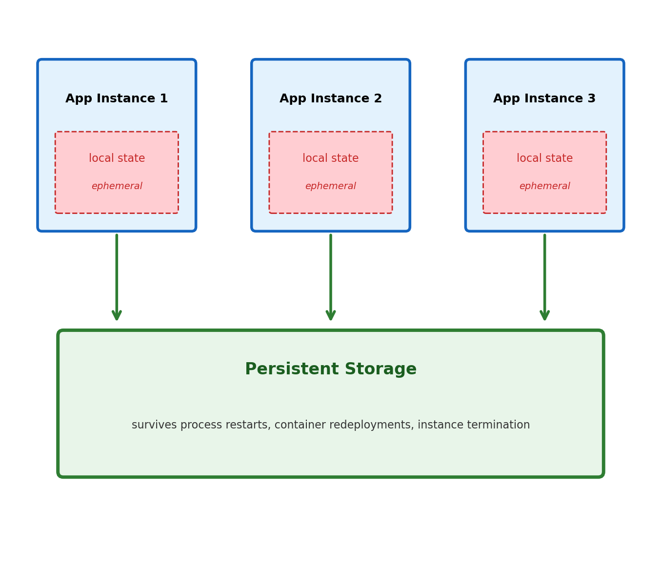
This is by design — stateless processes are straightforward to scale, replace, and restart. But the data they operated on must exist somewhere that outlives any individual process:
The actual records
The accumulated results
The shared state
Multiple Processes Need Access to the Same Data
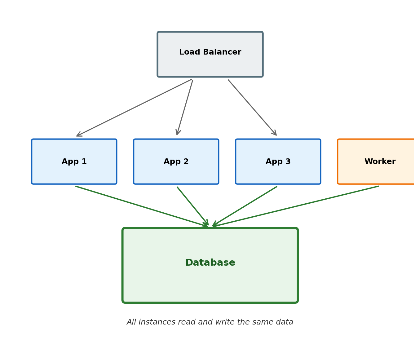
A typical application runs multiple instances of the same service behind a load balancer. Each instance handles a fraction of incoming requests.
Shared state is the norm, not the exception.
User A creates an account through instance 1. User B looks up that account through instance 3. Both need access to the same user record.
A background worker processes jobs queued by the web tier. The worker reads data the web tier wrote.
Example: an airline booking system runs 20 application servers. All 20 must see the same seat map — a seat sold through one instance must immediately be unavailable to all others.
Each process cannot maintain its own copy. Copies diverge immediately under concurrent writes. Reconciling divergent copies is one of the hardest problems in distributed systems.
Durable Writes Survive the Process That Made Them
Data written to a persistent store must survive the failure of the process that wrote it — a stronger guarantee than “data is saved to a file.”
Process crash — the application segfaults mid-operation. A kill -9 terminates it without cleanup. Completed writes are still present when the replacement process starts.
Container restart — a deployment rolls out new code. The orchestrator terminates the old container and starts a new one. Data written by the old version is available to the new version without any migration step.
Host failure — the physical server loses power. The disk may have had buffered writes that never been persisted. After recovery, committed data is intact because the database wrote it to a transaction log before acknowledging the commit.
An application that writes to a local file and calls flush() has no guarantee the data reached disk — the OS may buffer it. Databases use write-ahead logging (WAL) to close this gap: the commit is not acknowledged until the log entry is on stable storage.
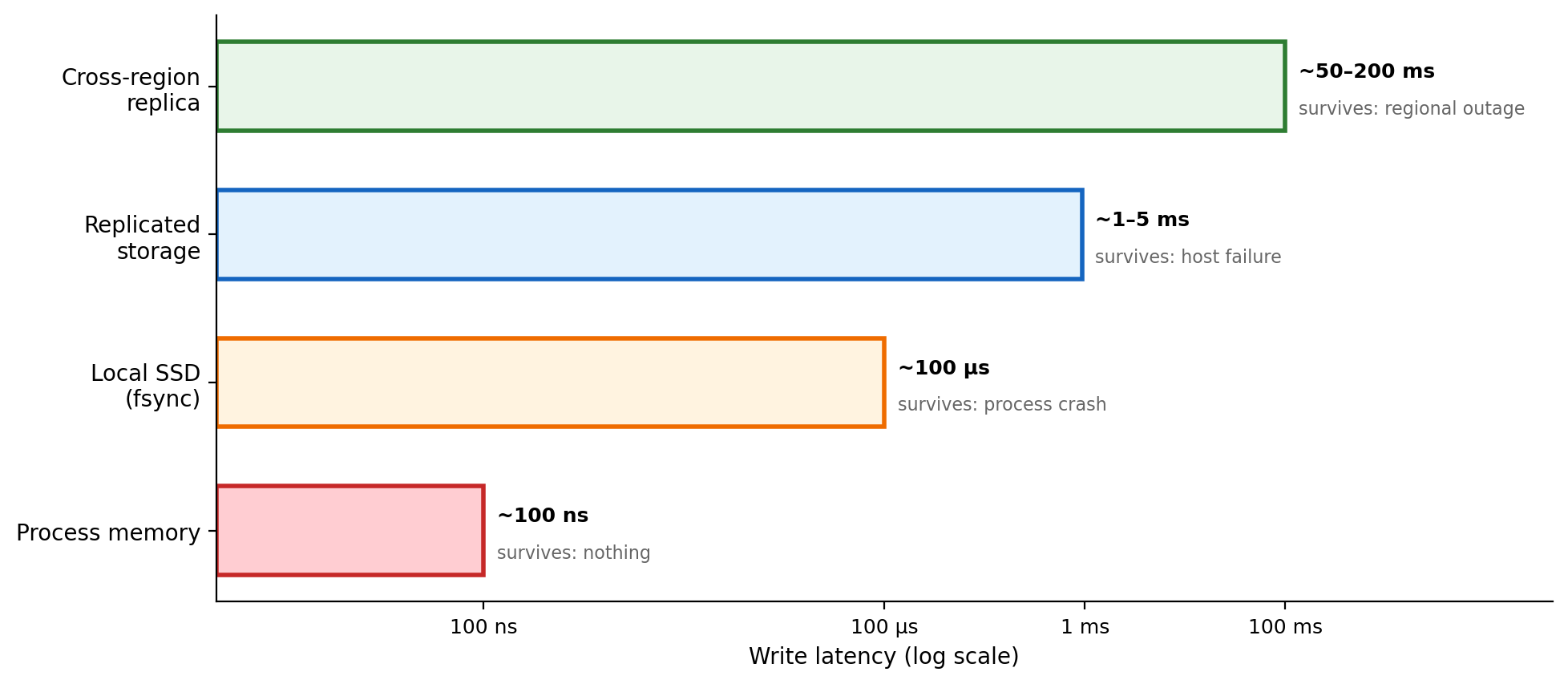
Durability Has Measurable Cost
Every level of durability corresponds to a specific mechanism. Stronger guarantees cost more time.
The gap between process memory (~100 ns) and a cross-region replica (~100 ms) is six orders of magnitude. A write that takes nanoseconds locally takes hundreds of milliseconds to guarantee survival of a regional outage.
Higher durability adds latency cost.
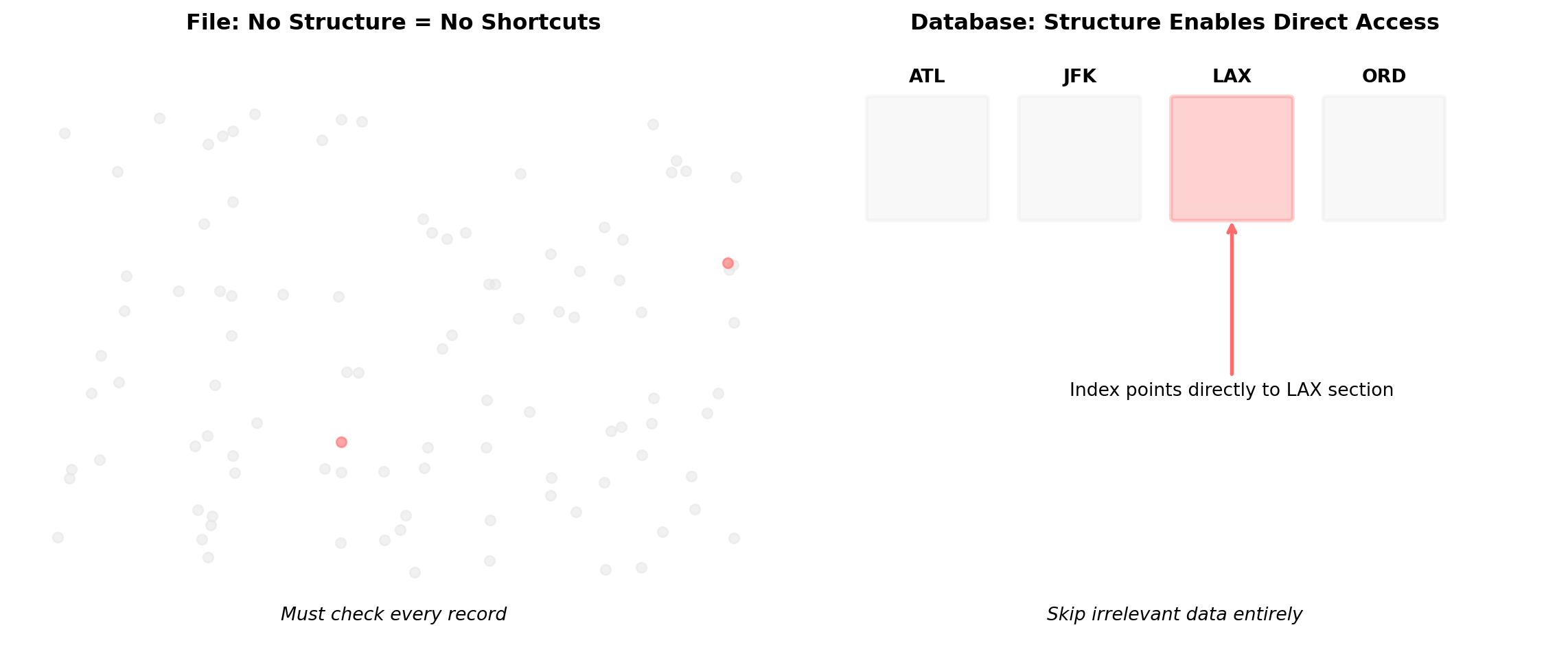
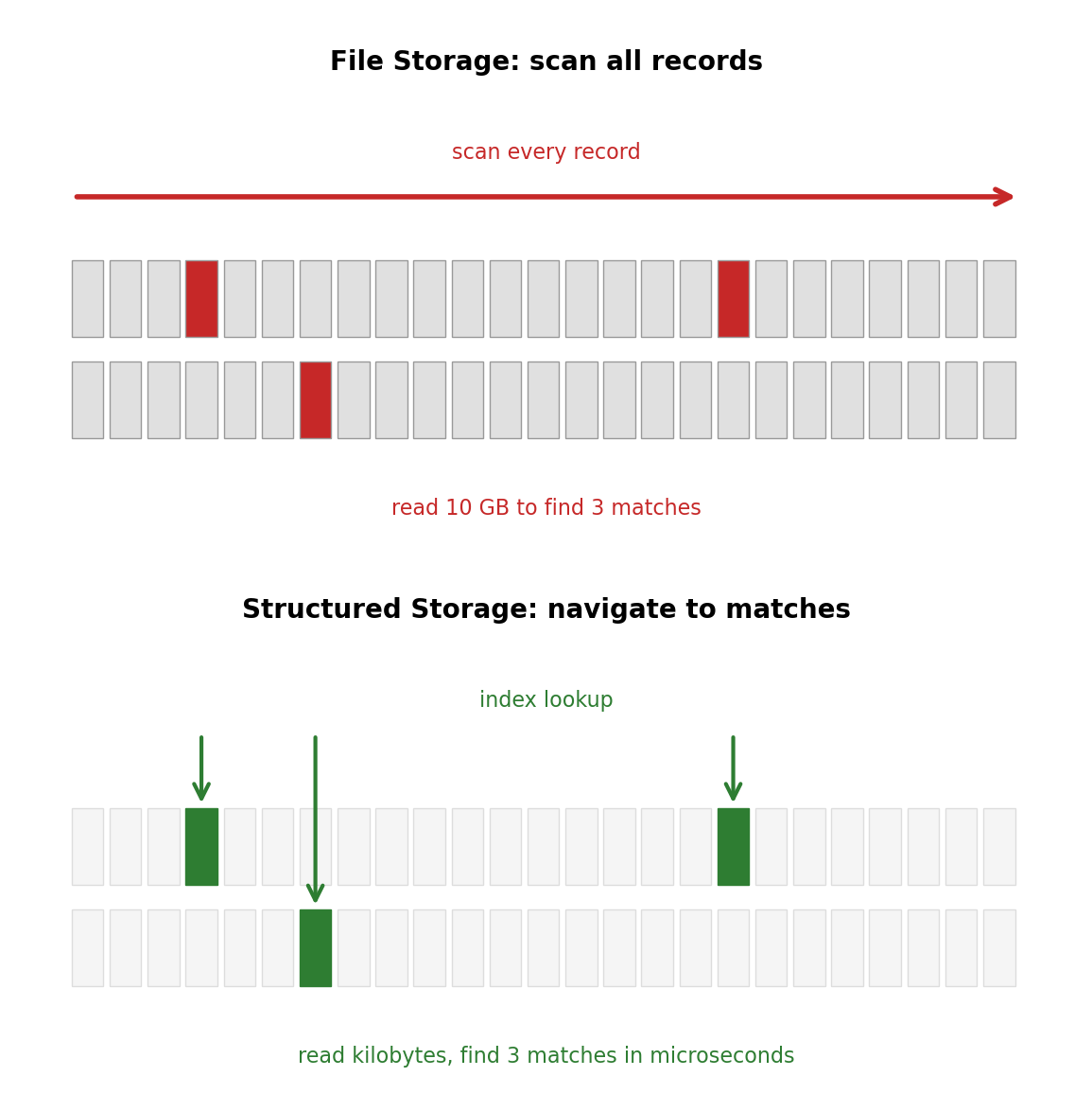
Unstructured Storage Forces Full Scans
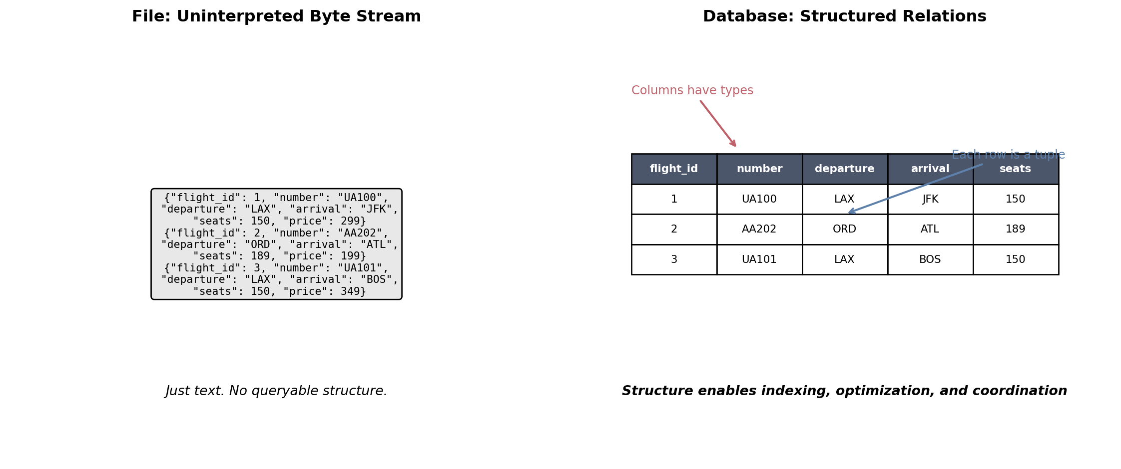
An application that stores flight records as flat files — one JSON blob per flight, or a single CSV — must read and parse the entire dataset to answer any question about it.
File or object storage retrieves by name.
# S3: retrieve a known objects3.get_object(Bucket='flights', Key='2026/02/lax-jfk.json')# Filesystem: read a known fileopen('/data/flights/2026/02/lax-jfk.json')
The application must know which object to retrieve. There is no mechanism to ask the storage system for objects matching a condition.
“Which flights from LAX have available seats?”
Download all flight objects
Parse each one (JSON decode, CSV parse)
Filter in application code
10 million records at 1 KB each = 10 GB transferred and parsed
The cost scales linearly with total data size, regardless of how selective the question is.
Structured Storage Knows the Shape of the Data
The storage system itself understands column names, types, and constraints. This knowledge is what enables selective access.
The database reads only matching records. With an index on (origin, departure_date), this touches a handful of disk pages regardless of total table size.
10 million records, same question: microseconds, reading kilobytes.
The database can do this because it knows:
origin is a character column with an index
departure_date is a date type, comparable with =
seats_remaining is an integer, comparable with >
The table has statistics on value distribution that inform which access strategy is cheapest
Without database-level structure, every application is responsible for:
Parsing and validating every record on read
Ensuring consistency across related records
Implementing its own search and filtering
Preventing concurrent writes from corrupting shared files
Every application that accesses the data re-implements this logic. Each implementation is an opportunity for divergence.
Application A reads a flight record as JSON with departure_time as an ISO-8601 string. Application B reads the same file and parses it as a Unix timestamp. Both are “correct” until a timezone mismatch causes a booking for the wrong flight.
A database centralizes these responsibilities. The structure is defined once, enforced by the storage system, and consistent for every client that connects.
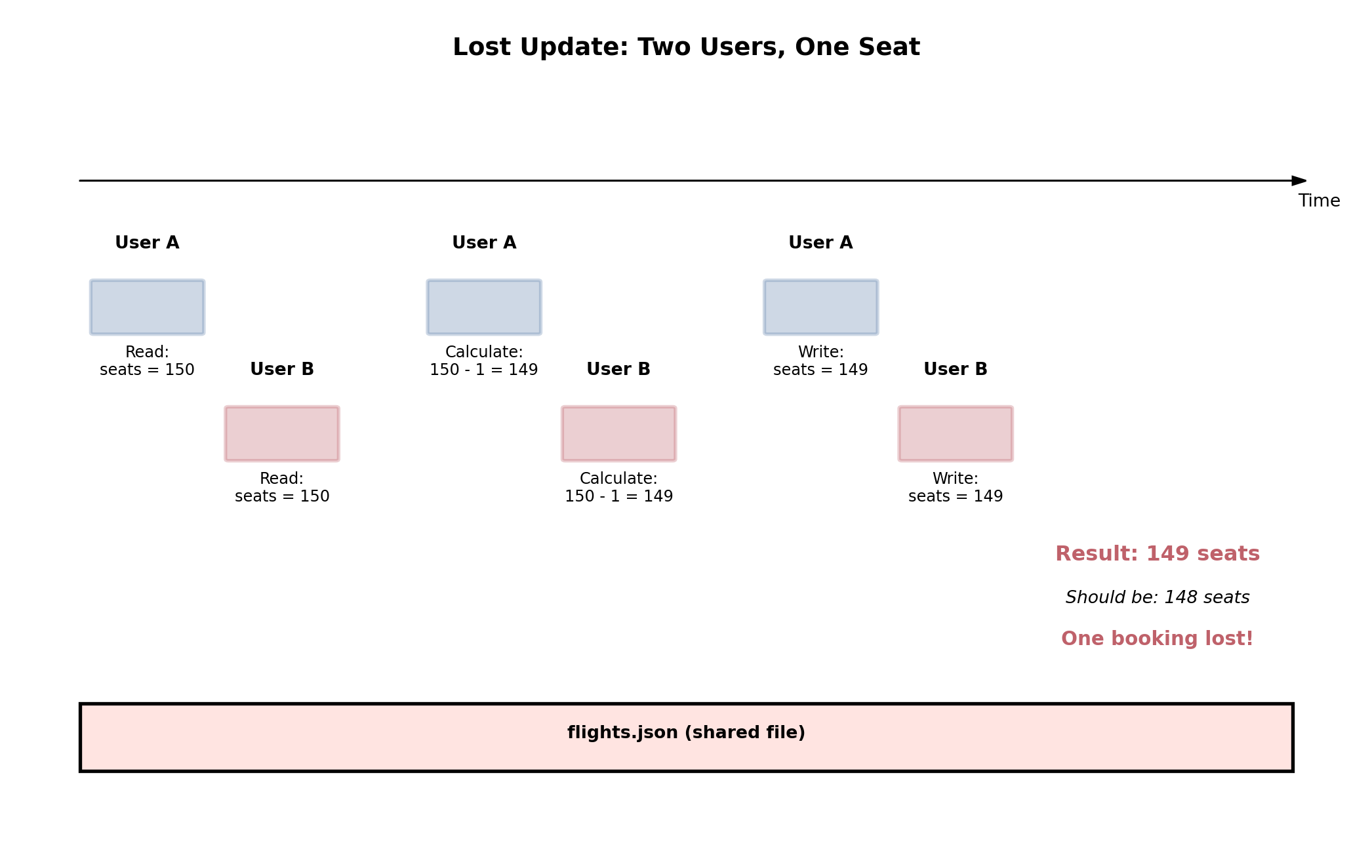
Concurrent Access Without Coordination Corrupts Data
Multiple processes writing to the same data simultaneously is the default operating condition for any shared storage system.
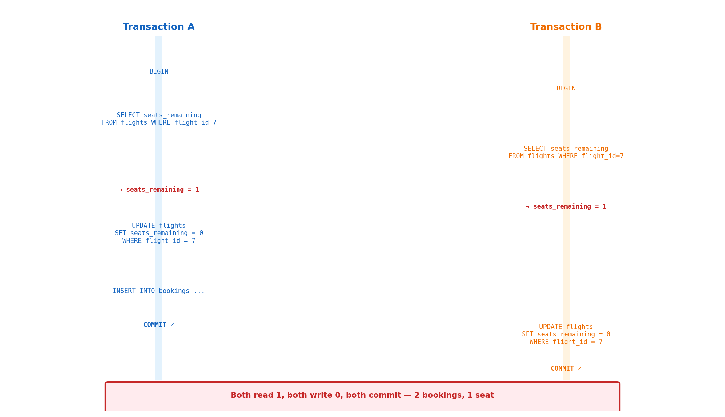
An airline booking system. Two users attempt to book the last seat on flight 547, at the same time, through different application servers:
App server A reads seat count: 1 remaining
App server B reads seat count: 1 remaining
App server A writes: 1 - 1 = 0 remaining, confirms booking
App server B writes: 1 - 1 = 0 remaining, confirms booking
Two confirmed bookings. One seat.
This is the lost update — a concurrency anomaly that occurs whenever read-then-write operations are not atomic. Both servers read the same value, both compute the same result, and the second write silently overwrites the first.
The anomaly is not caused by a bug in application logic. The code is correct for a single-writer system. It fails because the system has multiple writers and no coordination between them.
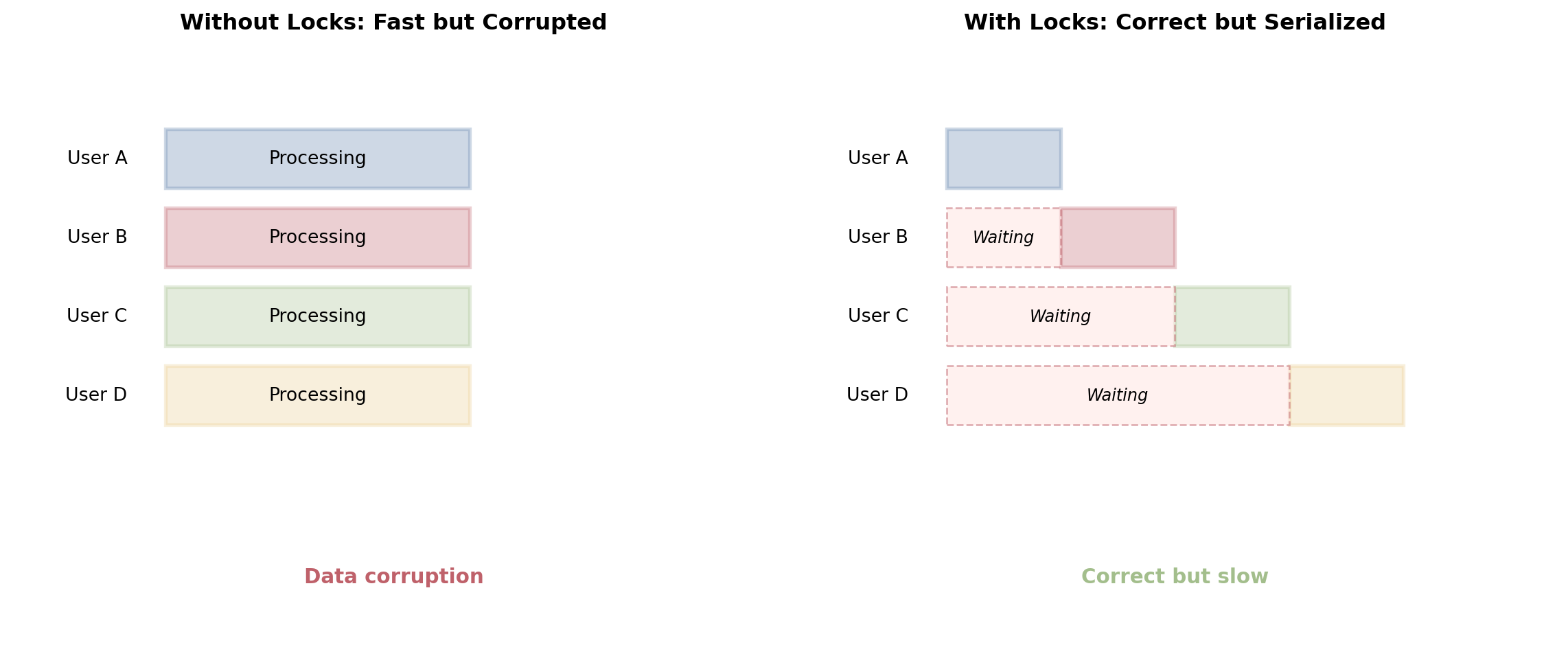
File Locking Does Not Scale
One workaround is file locking — flock() on Unix, LockFileEx() on Windows. One writer at a time.
File-level locking:
Lock the entire flights file
Read the seat count
Update and write back
Release the lock
This serializes all access. While one process holds the lock, every other process waits — including processes operating on completely unrelated flights.
A system with 10,000 flights and 100 concurrent users: every operation on every flight waits for a single global lock. Throughput falls.
Database row-level locking:
Lock only the row for flight 547
Other flights are unaffected
Processes operating on different flights proceed concurrently
The lock is held for milliseconds, not for the duration of a file I/O operation
Databases provide granular locking — down to individual rows — combined with transaction isolation that controls what concurrent readers can see. The coordination cost is proportional to actual contention, not to dataset size.
Replicating granular locking and transaction isolation on top of file storage means re-implementing substantial portions of a database engine.
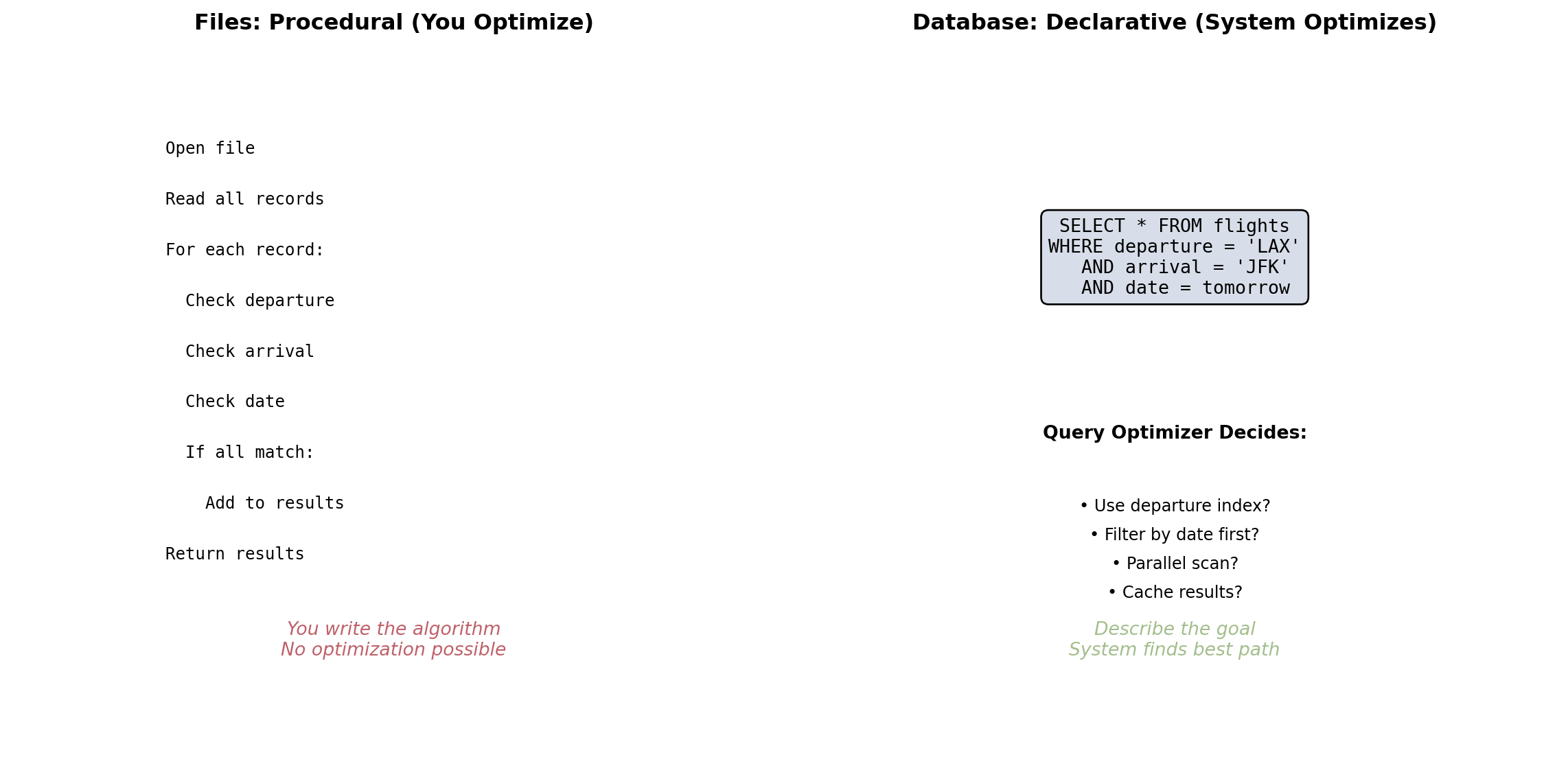
Procedural Data Access Binds Logic to Execution Strategy
When the application controls how data is accessed, the access strategy is embedded in the code.
# Find available flights from LAX on Feb 12results = []for flight in all_flights: # iterate every recordif flight['origin'] =='LAX'\and flight['seats'] >0\and flight['date'] =='2026-02-12': results.append(flight)
The strategy is fixed:
Sequential scan — always reads every record
Application bears the full cost of filtering
If data grows 100x, this code runs 100x slower
No way to use indexes, caches, or pre-sorted data without rewriting the loop
Changing access patterns requires changing code:
Want to speed up LAX lookups? Build an in-memory dictionary keyed by origin. Rewrite the query logic.
Want to support date-range queries? Sort the data by date. Rewrite again.
Want to join flights with bookings? Nested loops, careful key matching. More code, more bugs.
Every performance improvement is a code change. Every code change is a testing and deployment cycle.
Declarative Queries Let the Database Choose the Strategy
SQL specifies what data to return, not how to find it.
The query optimizer evaluates execution strategies:
No index on origin? Sequential scan.
Index on origin exists? Index lookup, then filter.
Index on (origin, departure_date)? Composite index lookup — reads only the exact set of matching rows.
Same SQL. The optimizer picks the cheapest plan based on:
Available indexes
Table size and row count estimates
Column value distribution (selectivity statistics)
Available memory for sorting and hashing
Performance improves without application changes.
An index is added on origin:
The optimizer detects the new index
Switches from sequential scan to index lookup
Query goes from scanning 10 million rows to reading a few hundred
No application code changes
This separation — application specifies intent, database chooses execution — is what allows databases to optimize independently of the applications that use them. It is the central architectural insight of the relational model.
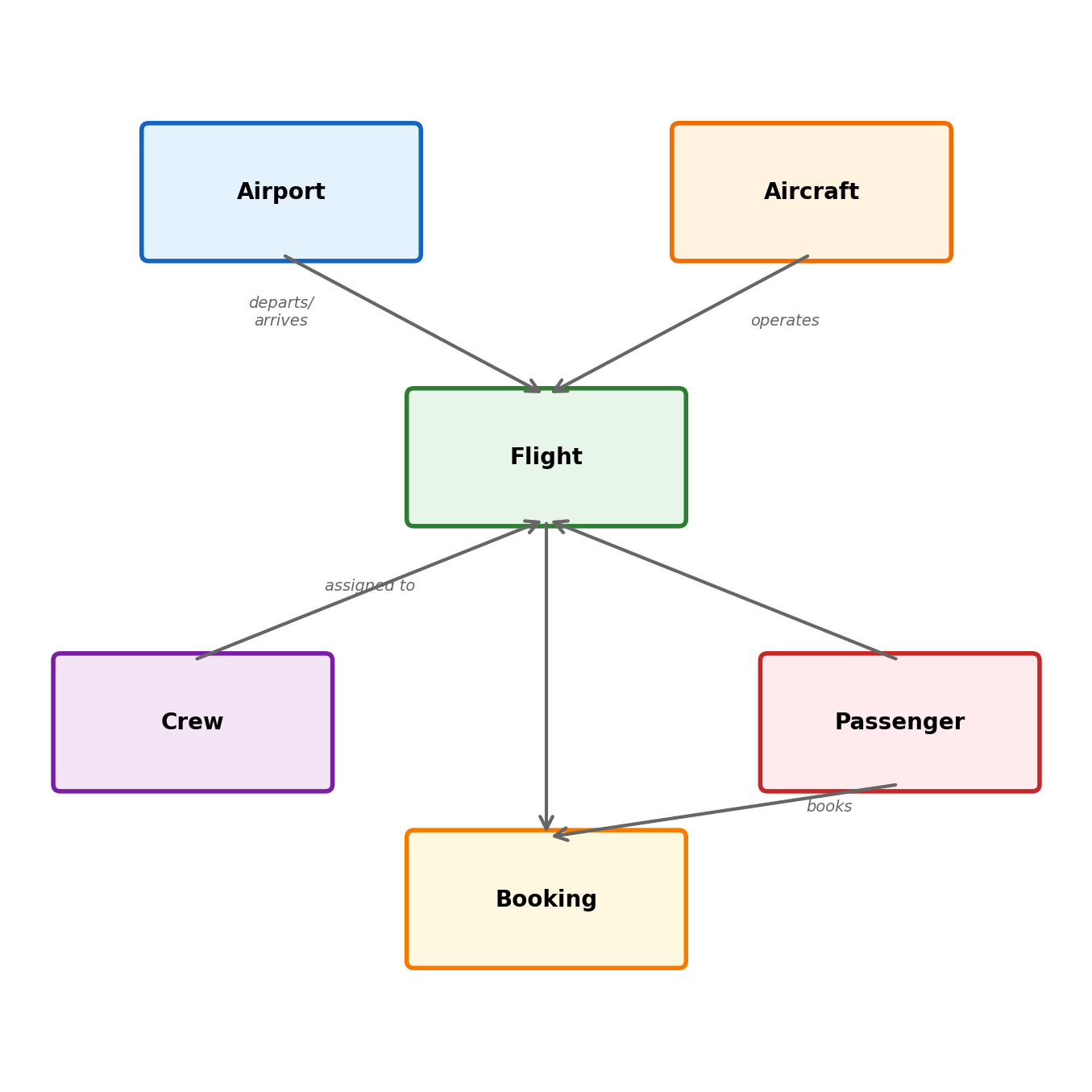
The Aviation Domain
An aviation domain: airlines, airports, flights, aircraft, crews, passengers, and bookings.
Core entities:
Airports — code, name, city, timezone
Aircraft — registration, model, seat capacity, range
Bookings — passenger, flight, seat, fare class, status
Relationships:
A flight departs from one airport, arrives at another
A flight is operated by one aircraft
A flight has multiple crew members (many-to-many)
A booking connects a passenger to a flight
An aircraft has a maintenance history
Typed columns — timestamps, airport codes
Constraints — a flight must reference existing airports
Relationships — many-to-many crew assignments
Concurrency — seat booking races
The Relational Model
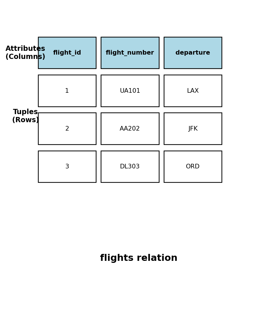
Data Organized into Tables
A relational database stores data in tables. Each table has a fixed set of columns with defined names and types. Each row is one record conforming to that structure.
flight_id
flight_number
origin
destination
departure_time
seats_remaining
1
AA 100
LAX
JFK
2026-02-12 08:00
23
2
UA 512
SFO
ORD
2026-02-12 09:30
0
3
DL 47
ATL
LAX
2026-02-12 11:15
84
This is not a spreadsheet. The structure is enforced:
Every row has the same columns
Every column has a declared type
The database rejects data that violates the structure
A row without a flight_number is not allowed (NOT NULL)
A departure_time value of "next Thursday" is rejected — the column expects a timestamp
Types Restrict What Values a Column Can Hold
Column types are not annotations — they are enforced constraints. The database rejects operations that violate them.
Common types:
INTEGER — whole numbers (flight_id, seat count)
TEXT / VARCHAR(n) — character strings, optionally length-limited
NUMERIC(p, s) — exact decimal with defined precision (monetary values, coordinates)
UUID — 128-bit universally unique identifier
Type choice has consequences:
NUMERIC(10,2) for currency — floating-point arithmetic introduces rounding errors that are unacceptable for financial calculations
TIMESTAMP WITH TIME ZONE for departure times — a flight departing LAX at 08:00 Pacific is not the same instant as 08:00 Eastern
CHAR(3) for airport codes — fixed length enforces the IATA standard
What the database rejects:
-- Type mismatch: text in an integer columnINSERTINTO flights (seats_total) VALUES ('many');-- ERROR: invalid input syntax for type integer-- Constraint violation: string too long for CHAR(3)INSERTINTO flights (origin) VALUES ('Los Angeles');-- ERROR: value too long for type character(3)-- Precision overflowINSERTINTO fares (price) VALUES (999999999.99);-- ERROR: numeric field overflow
The database enforces these at write time, not read time. Invalid data never enters the table. Every application that queries this table can rely on seats_total being an integer and origin being exactly 3 characters.
Contrast with JSON in a file: any value can appear in any field, and validation is the caller’s responsibility.
Every Row Needs an Identity
A table with duplicate rows is ambiguous. Which row should be updated? Which row was deleted? Without identity, operations on individual records are undefined.
Primary keys provide identity.
A primary key is a column (or combination of columns) whose value uniquely identifies each row. The database enforces two rules:
Uniqueness — no two rows can have the same primary key value
NOT NULL — the primary key cannot be absent
CREATETABLE airports ( airport_code CHAR(3) PRIMARYKEY, name TEXT NOTNULL, city TEXT NOTNULL, timezone TEXT NOTNULL);
airport_code uniquely identifies each airport. Inserting a second row with 'LAX' is rejected. Inserting a row with no airport code is rejected.
Most systems use surrogates for internal identity and natural keys as unique constraints
Foreign Keys Enforce Relationships Between Tables
Data about different entities lives in different tables. A flight has an origin airport and a destination airport. Rather than duplicating the airport name, city, and timezone in every flight row, the flight table references the airports table.
origin must contain a value that exists in airports.airport_code
Inserting a flight with origin = 'XYZ' fails if no airport XYZ exists
This is referential integrity — the database guarantees that every reference points to a real record
Attempting to insert an invalid reference:
INSERTINTO flights (origin, destination, ...)VALUES ('ZZZ', 'LAX', ...);-- ERROR: insert or update on table "flights"-- violates foreign key constraint-- Key (origin)=(ZZZ) is not present-- in table "airports"
What happens when the referenced row is deleted:
An airport is decommissioned. Flights still reference it. The database has three options, specified when the foreign key is created:
RESTRICT (default) — block the delete. Cannot remove an airport that flights reference.
CASCADE — delete the airport and all flights that reference it
SET NULL — delete the airport, set origin to NULL in referencing flights
Each represents a different business rule:
RESTRICT: airports cannot be removed while flights exist (most common)
CASCADE: removing an airport removes its flights (dangerous but appropriate in some contexts)
SET NULL: flights become “orphaned” with unknown origin (rarely desirable)
References Eliminate Redundant Data
Without foreign keys: data duplicated in every row
flight
origin_code
origin_name
origin_city
origin_tz
AA 100
LAX
Los Angeles International
Los Angeles
America/Los_Angeles
UA 200
LAX
Los Angeles International
Los Angeles
America/Los_Angeles
DL 300
LAX
Los Angeles International
Los Angeles
America/Los_Angeles
The airport name, city, and timezone are repeated for every flight from LAX. If LAX changes its name (it was renamed in 2017), every flight row must be updated. Miss one and the data is inconsistent.
With 10,000 flights from LAX, the name "Los Angeles International" is stored 10,000 times.
With foreign keys: stored once, referenced by code
airports:
airport_code
name
city
timezone
LAX
Los Angeles International
Los Angeles
America/Los_Angeles
flights:
flight_number
origin
destination
AA 100
LAX
JFK
UA 200
LAX
ORD
DL 300
LAX
ATL
Airport name stored once. Flights reference it by code. Name change: update one row in the airports table. All flights reflect the change immediately.
This principle — each fact stored once — is the foundation of normalization, developed in detail later.
Constraints Express Business Rules in the Schema
Beyond keys and types, the database can enforce arbitrary conditions on data.
NOT NULL — a value must be provided
flight_number TEXT NOTNULL
A flight without a flight number cannot exist. The database rejects the insert rather than storing an incomplete record.
UNIQUE — no duplicates allowed
aircraft_registration TEXT UNIQUE
No two aircraft can share a registration number. Unlike a primary key, a UNIQUE column can be NULL (an aircraft awaiting registration).
DEFAULT — value when none is provided
booking_status TEXT DEFAULT'confirmed'
A new booking without an explicit status is automatically 'confirmed'.
The seat count cannot go negative. The database rejects any update that would set seats_remaining to -1. This prevents overselling at the storage layer, regardless of application logic.
CHECK (departure_time < arrival_time)
A flight cannot arrive before it departs. This catches data entry errors, application bugs, and timezone conversion mistakes before they become corrupt records.
These rules are enforced regardless of which application writes the data. No application can bypass them.
Constraints are Centralized Enforcement
Consider the alternative: every application validates independently.
The web application checks seats_remaining >= 0 before confirming a booking
The batch import tool checks seats_remaining >= 0 before loading flight data
The admin console checks seats_remaining >= 0 before manual adjustments
A new mobile API is added six months later. The developer doesn’t know about the constraint. Negative seat counts enter the database.
Three applications enforced the rule correctly. The fourth didn’t. The data is now corrupt, and the source of the corruption is difficult to trace.
With a CHECK constraint on the column, the fourth application’s bad write is rejected at the database level. The rule is defined once, in the schema, and enforced universally.
NULL Represents Missing or Unknown Data
NULL is not zero. NULL is not an empty string. NULL is not false. NULL means the value is not known or does not apply.
When NULL is appropriate:
CREATETABLE flights (... actual_departure TIMESTAMP, -- NULL until takeoff gate_number TEXT, -- NULL if not assigned delay_minutes INTEGER-- NULL if on time);
A flight that hasn’t departed yet has no actual_departure. The value is genuinely unknown — not zero, not “1970-01-01”, not a placeholder. NULL is the correct representation.
When NULL is not appropriate:
flight_number TEXT NOTNULL-- every flight has a numberorigin CHAR(3) NOTNULL-- every flight has an origin
NOT NULL constraints prohibit NULL where absence would be nonsensical. A flight without an origin is not a flight.
NULL in expressions:
Any arithmetic or comparison with NULL yields NULL:
This is three-valued logic: TRUE, FALSE, NULL. Most languages have two truth values. SQL has three.
-- This finds NO rows where gate_number is NULLSELECT*FROM flights WHERE gate_number =NULL;-- This is correctSELECT*FROM flights WHERE gate_number ISNULL;
The first query compares each row’s gate_number with NULL. The comparison yields NULL, which is not TRUE, so no rows match — even the rows where gate_number is actually NULL.
NULL Propagation Affects Aggregation and Logic
Aggregation with NULLs:
-- delay_minutes: [10, NULL, 30, NULL, 20]SELECTCOUNT(*) FROM flights; -- 5SELECTCOUNT(delay_minutes) FROM flights; -- 3SELECTAVG(delay_minutes) FROM flights; -- 20.0
FALSE AND NULL is FALSE because regardless of the unknown value, the result is FALSE. TRUE OR NULL is TRUE for the same reason. But TRUE AND NULL is NULL — the result depends on the unknown value.
The Relational Model in One Table Definition
A CREATE TABLE statement that shows types, primary key, foreign keys, and constraints:
CREATETABLE bookings ( booking_id SERIAL PRIMARYKEY, passenger_id INTEGERNOTNULLREFERENCES passengers(passenger_id), flight_id INTEGERNOTNULLREFERENCES flights(flight_id), seat_number TEXT, fare_class CHAR(1) NOTNULLCHECK (fare_class IN ('F', 'J', 'W', 'Y')), booking_time TIMESTAMPWITHTIMEZONENOTNULLDEFAULT now(), status TEXT NOTNULLDEFAULT'confirmed'CHECK (status IN ('confirmed', 'cancelled', 'checked_in', 'boarded')),UNIQUE (flight_id, seat_number));
Identity and references:
booking_id — surrogate key, auto-generated
passenger_id — must reference an existing passenger
flight_id — must reference an existing flight
Neither reference can be NULL — a booking without a passenger or flight is meaningless
Constraints as business rules:
fare_class is one of F (first), J (business), W (premium economy), Y (economy) — no other values accepted
status follows a defined lifecycle — no arbitrary strings
(flight_id, seat_number) is UNIQUE — two passengers cannot occupy the same seat on the same flight
seat_number can be NULL — seat assigned later
booking_time defaults to the current timestamp
The Aviation Schema
Four tables, connected by foreign keys. We will use this this as our working schema for the lecture.
Flights cannot reference nonexistent airports or aircraft
Bookings cannot reference nonexistent flights
Seat counts cannot go negative
Fare classes restricted to valid codes (F/J/W/Y)
No duplicate seat assignments per flight
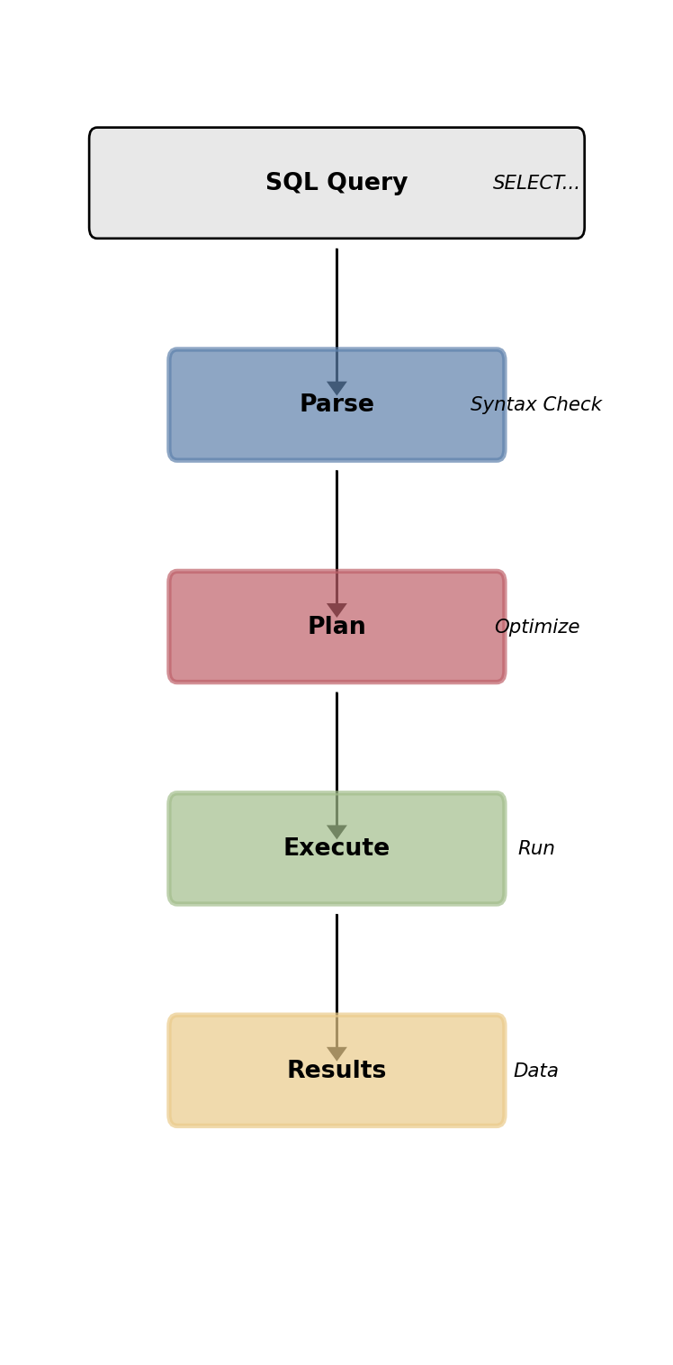
SQL
SQL Describes What, Not How
SQL is a declarative language. A query specifies the result — which rows, which columns, what conditions — and the database determines how to produce it.
SELECT*-- all columnsSELECT flight_number -- one columnSELECT flight_number, origin -- multiple columnsSELECTDISTINCT origin -- unique values only
FROM — which table (or tables) to read
FROM flightsFROM flights f -- alias for brevity in joins
WHERE — which rows to include
WHERE origin ='LAX'WHERE seats_remaining >0WHERE origin ='LAX'AND destination ='JFK'WHERE origin IN ('LAX', 'SFO', 'SEA')WHERE departure_time BETWEEN'2026-02-12'AND'2026-02-13'WHERE flight_number LIKE'AA%'-- starts with AAWHERE gate_number ISNULL-- no gate assignedWHERE gate_number ISNOTNULL-- gate assigned
Each condition is a predicate. Predicates combine with AND, OR, and NOT. The database evaluates them against each row and returns those where the overall expression is TRUE.
SQL Execution Order Differs from Written Order
A query is written SELECT ... FROM ... WHERE ... GROUP BY ... ORDER BY, but the database evaluates clauses in a different order.
Why this matters:
Column alias defined in SELECT cannot be used in WHERE — SELECT hasn’t executed yet
HAVING can filter on aggregates, WHERE cannot — WHERE executes before GROUP BY
ORDER BY can use SELECT aliases — it runs after SELECT
ORDERBY departure_time -- ascending (default)ORDERBY departure_time ASC-- explicit ascendingORDERBY departure_time DESC-- descendingORDERBY origin, departure_time -- sort by origin first,-- then by time within origin
Without ORDER BY, the database returns rows in whatever order is cheapest to produce. That order is not guaranteed and may change between executions.
LIMIT — restrict result count
LIMIT10-- first 10 rowsLIMIT10 OFFSET 20-- rows 21-30
LIMIT without ORDER BY returns an arbitrary subset — which 10 rows is undefined.
Present: the booking exists, which passenger, which flight, which seat.
Absent: passenger name, flight number, origin, destination, departure time — all in other tables.
To answer “passenger 42’s itinerary with flight details and airport names” requires combining four tables: bookings, flights, and airports (twice — origin and destination).
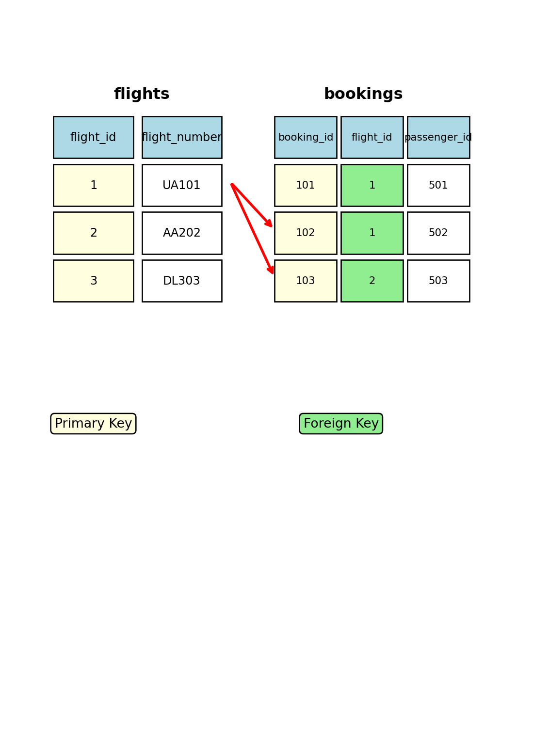
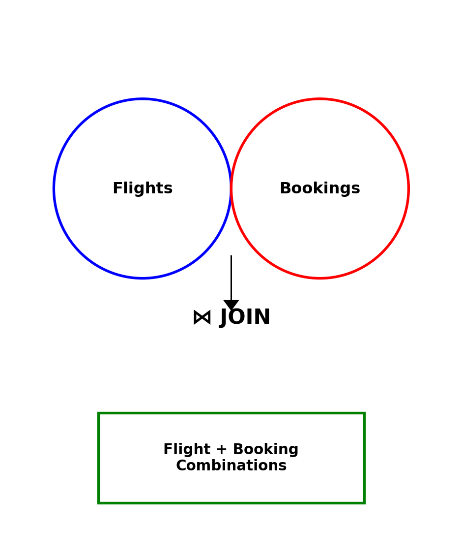
JOIN Matches Rows Across Tables
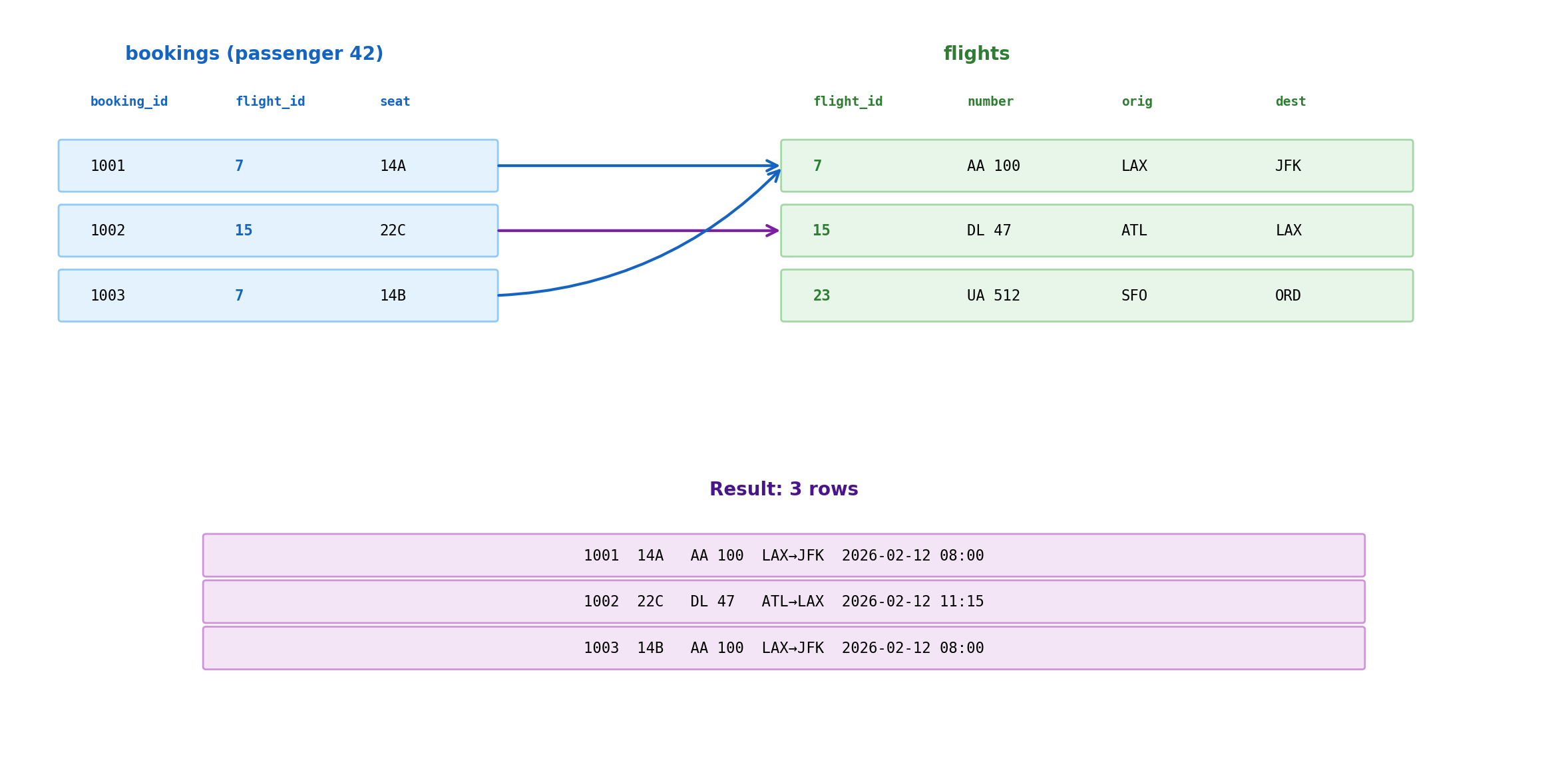
A JOIN combines rows from two tables based on a matching condition. For each row in the first table, the database finds rows in the second table where the condition holds, and produces a combined output row.
SELECT b.booking_id, b.seat_number, f.flight_number, f.departure_timeFROM bookings bJOIN flights f ON b.flight_id = f.flight_idWHERE b.passenger_id =42;
FROM bookings b — start with booking rows for passenger 42
JOIN flights f — for each booking, find the flight where flight_id matches
ON b.flight_id = f.flight_id — the match condition (foreign key = primary key)
Result: one row per booking, with flight details attached
Bookings 1001 and 1003 both match flight 7 — two passengers on the same flight, two result rows
Flight 23 has no bookings from passenger 42 — excluded from the result
One-to-many: one flight, many bookings. The join produces one output row per booking, not per flight
The JOIN Condition Controls Matching
JOIN flights f ON b.flight_id = f.flight_id
The ON clause specifies how rows from the two tables relate — typically a foreign key in one table matching a primary key in the other.
Every booking paired with every flight. 1,000 bookings × 10,000 flights = 10 million rows. Almost all meaningless.
The ON clause filters the cross product down to only meaningful pairs — rows where the foreign key actually matches.
ON as a filter on the cross product:
bookings.flight_id
flights.flight_id
match?
7
7
yes → include
7
15
no → discard
7
23
no → discard
15
7
no → discard
15
15
yes → include
15
23
no → discard
6 possible pairs → 2 matches
In production, the optimizer never materializes the full cross product — it uses indexes and hash tables to find matches directly.
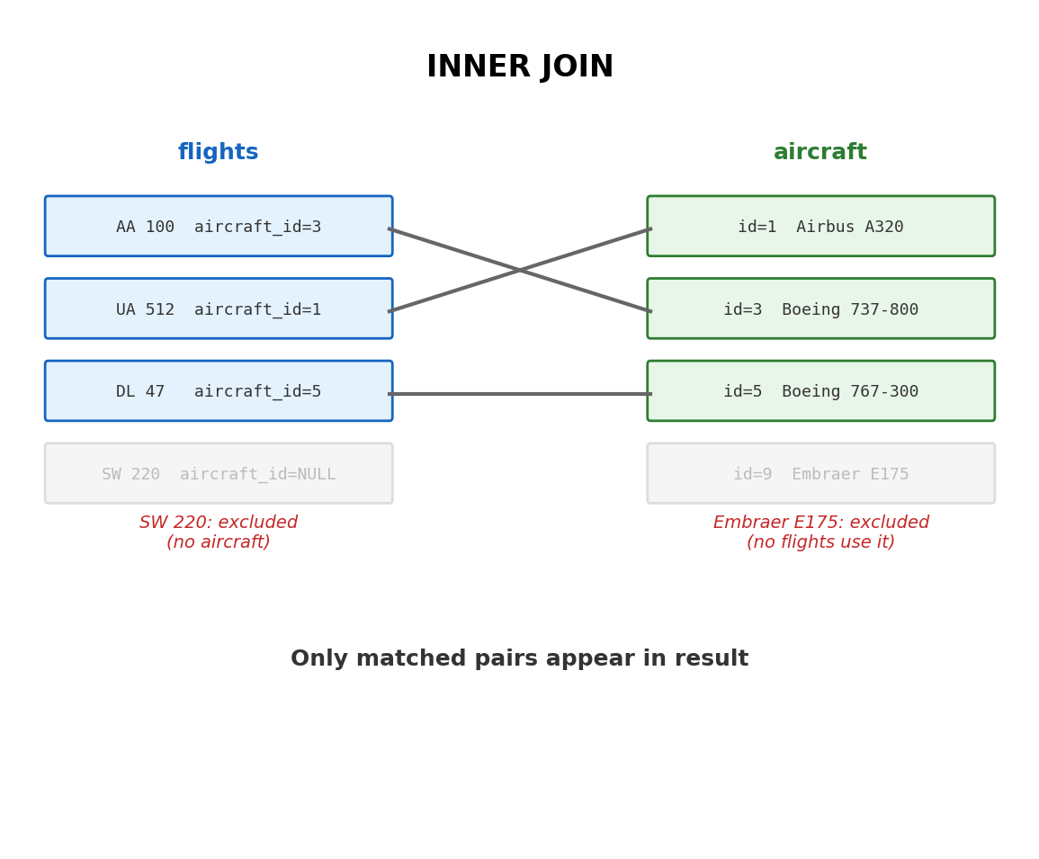
INNER JOIN Returns Only Matching Rows
The default JOIN (also written INNER JOIN) includes a row in the result only if a match exists in both tables.
SELECT f.flight_number, a.model AS aircraftFROM flights fJOIN aircraft a ON f.aircraft_id = a.aircraft_id;
flight_number | aircraft
--------------+-----------------
AA 100        | Boeing 737-800
UA 512        | Airbus A320
DL 47         | Boeing 767-300
500 flights, 20 have no aircraft assigned (aircraft_id is NULL). The result has 480 rows. The 20 unassigned flights are excluded — no match in the aircraft table.
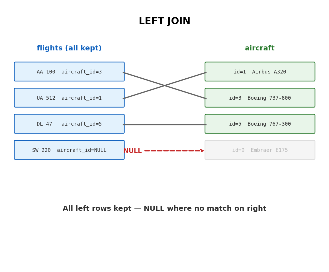
LEFT JOIN Preserves All Rows from the Left Table
LEFT JOIN returns every row from the left table. Where a match exists in the right table, the columns are filled. Where no match exists, the right-side columns are NULL.
SELECT f.flight_number, a.model AS aircraftFROM flights fLEFTJOIN aircraft a ON f.aircraft_id = a.aircraft_id;
flight_number | aircraft
--------------+-----------------
AA 100        | Boeing 737-800
UA 512        | Airbus A320
DL 47         | Boeing 767-300
SW 220        | NULL
All 500 flights appear — including the 20 with no aircraft assignment. The aircraft column is NULL for those rows.
Joining Multiple Tables
Each JOIN adds one more table to the result, matching on its own condition. Chains of joins follow the foreign key relationships through the schema.
SELECT b.booking_id, b.fare_class, b.seat_number, f.flight_number, f.departure_time, a_orig.name AS origin_airport, a_dest.name AS destination_airportFROM bookings bJOIN flights f ON b.flight_id = f.flight_idJOIN airports a_orig ON f.origin = a_orig.airport_codeJOIN airports a_dest ON f.destination = a_dest.airport_codeWHERE b.passenger_id =42;
The join chain:
bookings — start with passenger 42’s bookings
→ flights — match each booking to its flight via flight_id
→ airports as a_orig — resolve origin code to airport name
→ airports as a_dest — resolve destination code to airport name
The airports table appears twice with different aliases — a flight references two different airports. Aliases (a_orig, a_dest) disambiguate which role each join fills.
booking | fare | seat | flight | departure        | origin           | dest
--------+------+------+--------+------------------+------------------+-----------
1001    | Y    | 14A  | AA 100 | 2026-02-12 08:00 | Los Angeles Intl | John F. Kennedy
1002    | Y    | 22C  | DL 47  | 2026-02-12 11:15 | Hartsfield-Jksn  | Los Angeles Intl
Each result row assembles data from four tables:
booking_id, fare, seat — from bookings
flight, departure — from flights
origin, dest — from airports (two separate joins)
Joins Reassemble Normalized Data
Each fact stored once — airport name in one row, flight details in one row — reassembled by joins at query time.
The cost of reassembly: CPU and I/O to match rows across tables. Indexes on join columns (foreign keys, primary keys) keep this cost proportional to result size, not table size.
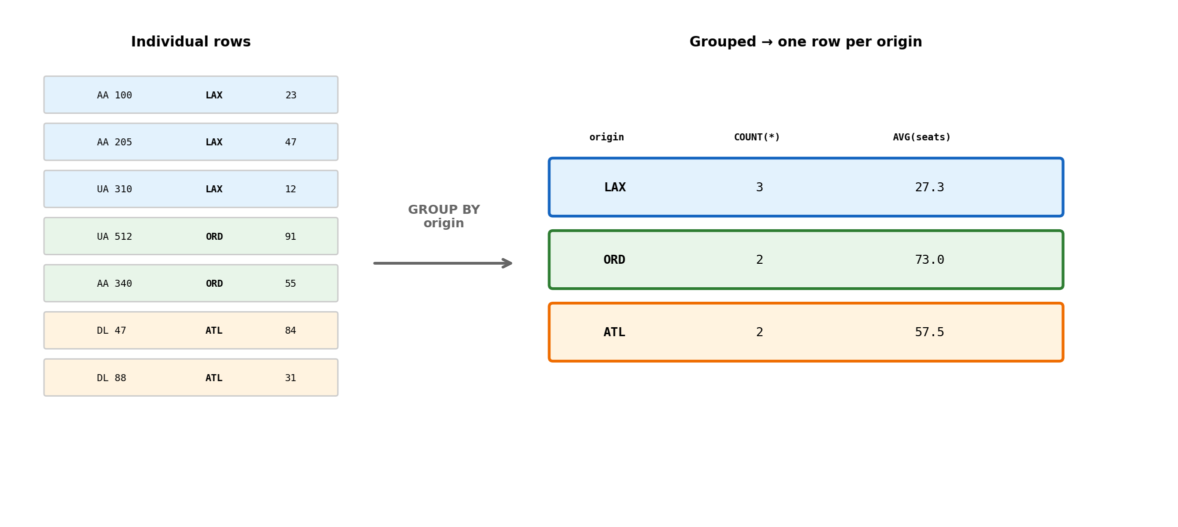
Aggregation: GROUP BY and Aggregate Functions
Aggregation computes summary values across sets of rows.
SELECT origin, COUNT(*) AS flight_count, AVG(seats_remaining) AS avg_seatsFROM flightsWHERE departure_time BETWEEN'2026-02-12'AND'2026-02-13'GROUPBY originORDERBY flight_count DESC;
Without GROUP BY, aggregates operate on the entire result set. With GROUP BY, they operate per-group.
WHERE vs HAVING:
WHERE filters individual rows before grouping. HAVING filters groups after aggregation.
SELECT origin, COUNT(*) AS flight_countFROM flightsWHERE departure_time >'2026-02-12'-- filter rowsGROUPBY originHAVINGCOUNT(*) >30; -- filter groups
“Airports with more than 30 flights tomorrow” — WHERE selects tomorrow’s flights, GROUP BY groups by origin, HAVING keeps only groups with more than 30.
GROUP BY Partitions Rows, Then Collapses Them
7 rows → 3 summary rows. The detail is gone — only the aggregates remain. GROUP BY answers “how many” and “what’s the average” but discards individual row identity.
Aggregation Across Joins
Aggregation and joins combine to answer questions that span multiple tables.
Bookings per airline for a given date:
SELECT substring(f.flight_number, 1, 2) AS airline,COUNT(b.booking_id) AS total_bookings,COUNT(DISTINCT f.flight_id) AS flightsFROM flights fJOIN bookings b ON f.flight_id = b.flight_idWHERE f.departure_time::date='2026-02-12'GROUPBY airlineORDERBY total_bookings DESC;
SELECT aggregates — count bookings and distinct flights per group
ORDER BY — sort by total bookings
COUNT(b.booking_id) — counts every booking row in the group
COUNT(DISTINCT f.flight_id) — counts unique flights only
23 flights, 1,247 bookings → ~54 passengers per flight
Subqueries and CTEs (advanced)
Complex questions often require composing queries — the result of one query becomes input to another.
Subquery — nested inside another query:
-- Flights with above-average bookingsSELECT f.flight_number, COUNT(b.booking_id) AS bookingsFROM flights fJOIN bookings b ON f.flight_id = b.flight_idGROUPBY f.flight_id, f.flight_numberHAVINGCOUNT(b.booking_id) > (SELECTAVG(booking_count) FROM (SELECTCOUNT(*) AS booking_countFROM bookings GROUPBY flight_id ) sub);
Reads inside-out:
Innermost — count bookings per flight
Middle — average those counts
Outer — keep flights above average
CTE (Common Table Expression) — same logic, reads top-to-bottom:
WITH per_flight AS (SELECT flight_id, COUNT(*) AS booking_countFROM bookingsGROUPBY flight_id),avg_bookings AS (SELECTAVG(booking_count) AS avg_countFROM per_flight)SELECT f.flight_number, pf.booking_countFROM per_flight pfJOIN flights f ON pf.flight_id = f.flight_idWHERE pf.booking_count > (SELECT avg_count FROM avg_bookings);
Each WITH clause defines a named intermediate result
CTEs can reference earlier CTEs
Main query uses them like tables
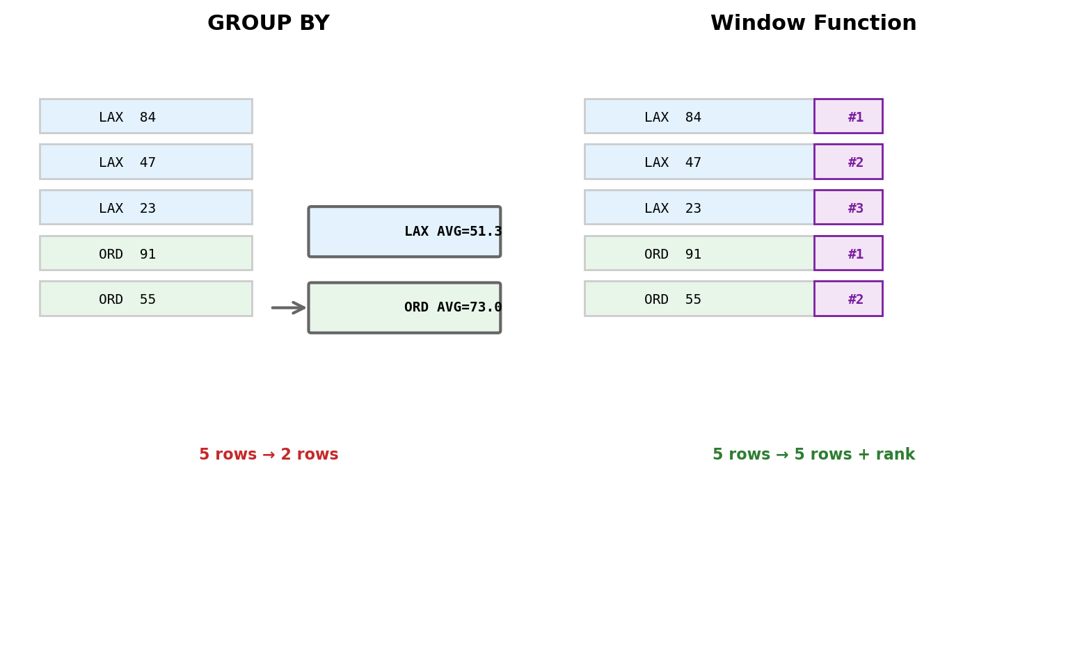
Window Functions (advanced)
GROUP BY collapses rows — one output per group, detail discarded. Window functions compute across related rows while preserving every row in the result.
SELECT flight_number, origin, seats_remaining,RANK() OVER (PARTITIONBY originORDERBY seats_remaining DESC ) AS availability_rankFROM flightsWHERE departure_time::date='2026-02-12';
flight_number | origin | seats | rank
--------------+--------+-------+-----
AA 100        | LAX    |    84 |    1
UA 205        | LAX    |    47 |    2
DL 300        | LAX    |    23 |    3
UA 512        | ORD    |    91 |    1
AA 340        | ORD    |    55 |    2
Every row is preserved. The rank is computed within each origin partition.
Common window functions:
ROW_NUMBER() / RANK() / DENSE_RANK() — numbering and ranking
Seq Scan on flights
Filter: (origin = ‘LAX’ AND departure_time > …)
Rows Removed by Filter: 9700
Actual Rows: 300
Sequential scan — reads every row, discards non-matches. Cost proportional to table size.
With an index on origin:
Index Scan using flights_origin_idx on flights
Index Cond: (origin = ‘LAX’)
Filter: (departure_time > …)
Actual Rows: 300
Index scan — navigates directly to LAX flights, then filters by date. Reads hundreds of rows instead of tens of thousands.
Same SQL, different plans. The optimizer switched strategy because an index became available. No application code changed.
Common plan nodes:
Seq Scan — full table read, O(n)
Index Scan — index lookup, O(log n)
Hash Join / Nested Loop — join strategies
Sort — explicit sort (ORDER BY)
Aggregate — GROUP BY computation
EXPLAIN ANALYZE — runs the query and reports actual times:
Planning Time: 0.2 ms
Execution Time: 1.3 ms
Schema Design and ER Modeling
Querying vs Designing
SQL operates on existing tables. Someone decided those tables exist, chose the columns, defined the types, and drew the foreign key relationships.
Schema design is that prior step: given a domain (“airlines, flights, passengers, bookings”), decide:
What entities need their own table
What attributes each entity has
How entities relate to each other
What constraints enforce correctness
Entity-Relationship (ER) modeling is a design tool for this process.
Visual notation for entities, attributes, and relationships
Independent of any specific database — a design artifact, not SQL
Forces decisions about cardinality (“can a flight have multiple aircraft?”) and participation (“must every aircraft be assigned to a flight?”) before writing DDL
The ER diagram is a blueprint; the CREATE TABLE statements are the implementation
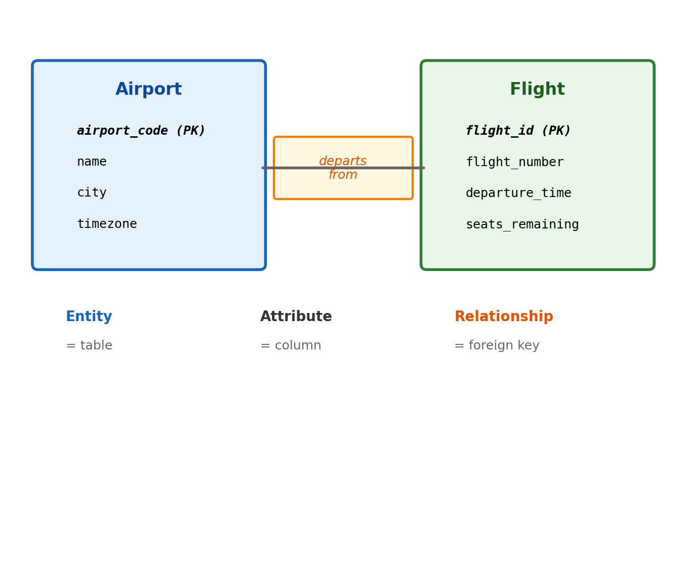
Entities, Attributes, Relationships
Entities — things with independent existence that the system needs to track.
Airport, Aircraft, Flight, Crew Member, Passenger
Each becomes a table
Has a primary key that provides identity
Attributes — properties of an entity.
Airport: code, name, city, timezone
Aircraft: registration, model, seat capacity, range
Each becomes a column with a type
Relationships — associations between entities.
A flight departs from an airport
A flight is operated by an aircraft
A passenger books a flight
Relationships are named — the verb matters for understanding direction and meaning
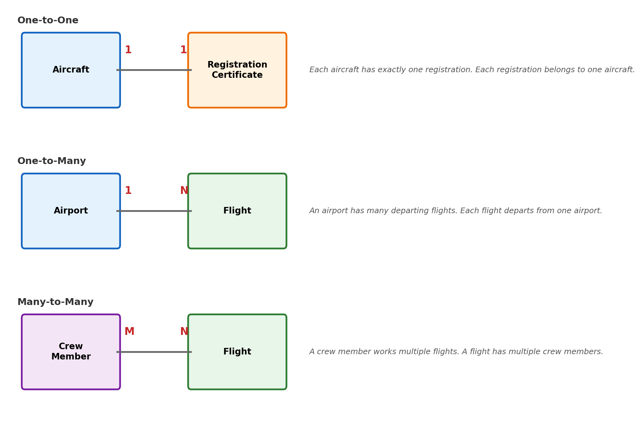
Cardinality: How Many on Each Side
Cardinality specifies how many instances of one entity can be associated with instances of another. This determines how the relationship is implemented in tables.
Cardinality Determines Implementation
One-to-many → foreign key in the “many” table
An airport has many flights. The foreign key goes in flights:
The foreign key lives in flights (the “many” side). The airport table has no reference back — the relationship is navigated from the many side.
One-to-one → foreign key with UNIQUE
CREATETABLE registration_certs ( cert_id SERIAL PRIMARYKEY, aircraft_id INTEGERUNIQUEREFERENCES aircraft(aircraft_id),...);
The UNIQUE constraint on aircraft_id enforces that no two certificates reference the same aircraft.
Many-to-many → junction table
Neither table can hold a single foreign key to the other — a crew member works multiple flights and a flight has multiple crew. A junction table represents the relationship:
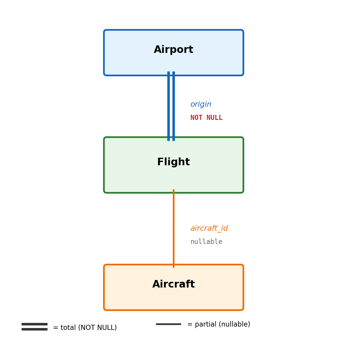
Partial participation — participation is optional.
An aircraft may or may not be assigned to a flight — new aircraft, or aircraft in maintenance
Implementation: foreign key allows NULL
aircraft_id INTEGERREFERENCES aircraft(aircraft_id)-- NULL means "not currently assigned"
Total participation → NOT NULL on the foreign key. Partial participation → nullable foreign key. The ER diagram captures the business rule; the DDL enforces it.
Weak Entities Depend on a Parent for Identity
Most entities are identified by their own attributes — an airport by its code, an aircraft by its registration. Weak entities have meaning only within the context of a parent.
A flight leg — one segment of a multi-stop flight:
Flight AA 100, Leg 1: LAX → DEN
Flight AA 100, Leg 2: DEN → JFK
“Leg 1” alone is not unique — every multi-stop flight has a “leg 1.” The leg is only identifiable as leg 1 of flight AA 100.
leg_number — identifies which leg within that flight (partial key)
Together: unique. Neither alone is sufficient.
Defining characteristics:
Cannot exist without the parent — deleting the flight deletes its legs (CASCADE)
Primary key includes parent’s key — identity depends on the parent
Identifying relationship — the parent contributes to identity, not just association
Other examples: line items on an invoice, rooms within a building, episodes within a season.
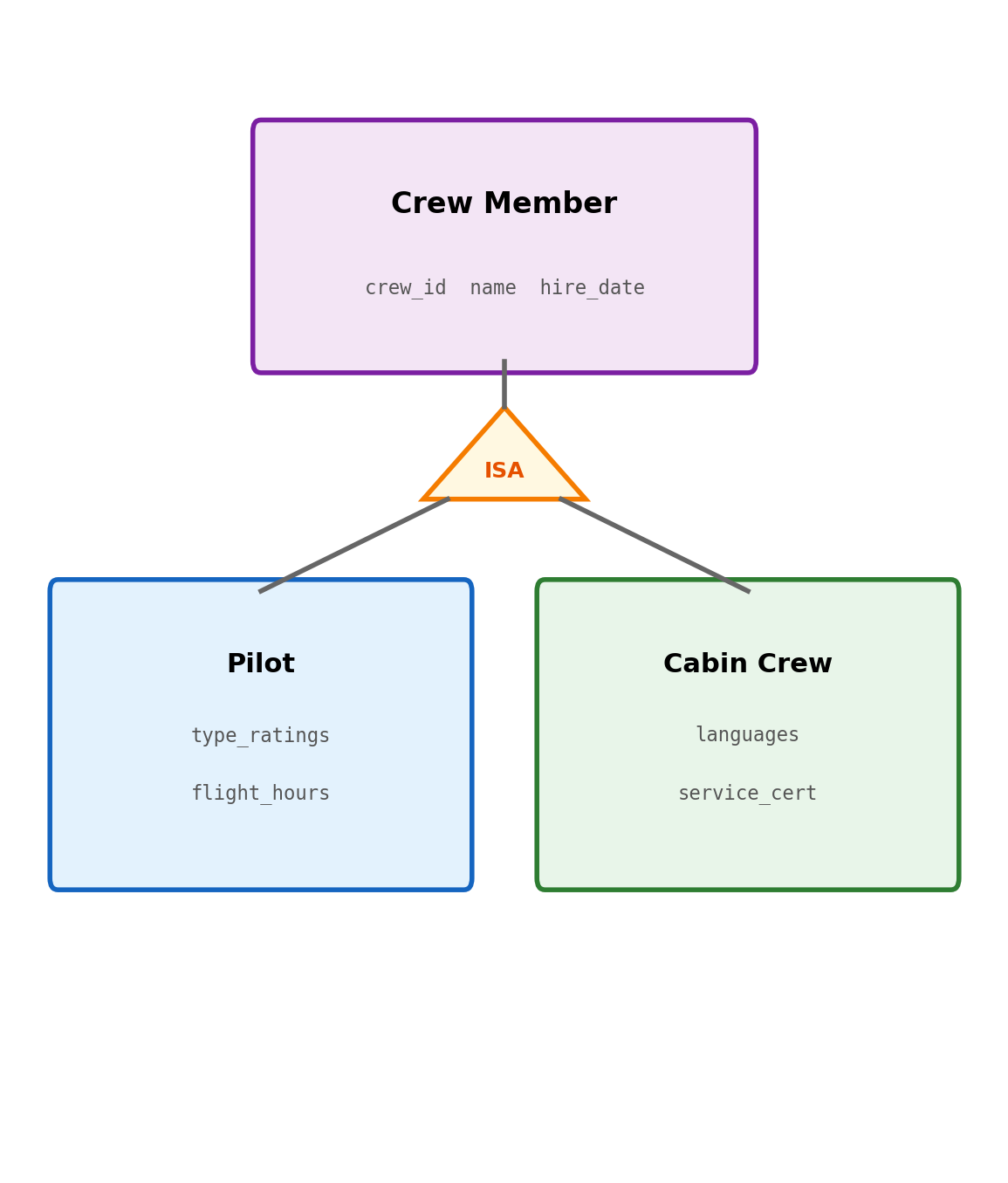
“ISA” Hierarchies: Specialization and Generalization
Some entities are subtypes of a more general entity. Crew members are all employees with shared attributes (name, employee ID, hire date), but pilots have type ratings and cabin crew have language certifications.
Implementation options:
Single table with type column:
CREATETABLE crew ( crew_id SERIAL PRIMARYKEY, name TEXT NOTNULL, hire_date DATENOTNULL, crew_type TEXT NOTNULLCHECK (crew_type IN ('pilot', 'cabin')), type_ratings TEXT[], -- NULL for cabin crew flight_hours INTEGER, -- NULL for cabin crew languages TEXT[], -- NULL for pilots service_cert TEXT -- NULL for pilots);
One table, simple queries, no joins
type_ratings is NULL for every cabin crew row
Inapplicable columns accumulate as subtypes diverge
Separate tables, shared primary key:
CREATETABLE crew ( crew_id SERIAL PRIMARYKEY, name TEXT NOTNULL, hire_date DATENOTNULL);CREATETABLE pilots ( crew_id INTEGERPRIMARYKEYREFERENCES crew(crew_id), type_ratings TEXT[], flight_hours INTEGER);CREATETABLE cabin_crew ( crew_id INTEGERPRIMARYKEYREFERENCES crew(crew_id), languages TEXT[], service_cert TEXT);
Each subtype holds only its own columns
JOIN required for shared + specific attributes
FK enforces subtype corresponds to real crew member
From Requirements to ER Diagram
Requirements (aviation booking system):
Airlines operate flights between airports
Each flight is operated by one aircraft
Flights have scheduled departure and arrival times
Crew members are assigned to flights; a flight has multiple crew
Passengers book flights
A booking records the passenger, flight, seat, and fare class
Aircraft have maintenance records
Entities identified:
Airport, Aircraft, Flight, Crew Member, Passenger, Booking, Maintenance Record
Relationships identified:
Flight departs from / arrives at Airport (many-to-one, total)
Flight operated by Aircraft (many-to-one, partial — aircraft may not be assigned yet)
Crew Member assigned to Flight (many-to-many)
Passenger makes Booking (one-to-many)
Booking for Flight (many-to-one, total)
Aircraft has Maintenance Record (one-to-many)
The Aviation ER Diagram
Cardinality summary:
Airport 1 — N Flight (one airport, many flights)
Aircraft 1 — N Flight (one aircraft, many flights)
The ER diagram forces decisions that affect every query, every constraint, and every future schema change.
“Can a booking exist without a flight?”
If yes: flight_id nullable, LEFT JOINs needed, application must handle orphaned bookings
If no: NOT NULL REFERENCES, database prevents orphaned bookings at write time
“Can two passengers share a seat?”
If no: UNIQUE(flight_id, seat_number) — enforced by the database, regardless of application logic
If yes (standby, etc.): no unique constraint, application manages conflicts
“Is fare class a free-text field or an enumeration?”
Free text: flexible, no validation, inconsistent values guaranteed over time ("economy", "Economy", "Y", "econ")
CHECK constraint: fare_class IN ('F','J','W','Y') — consistent, but requires schema change to add a new class
These decisions are difficult to change later.
Adding NOT NULL to a column with existing NULLs → data migration
Splitting a table → rewrite every query that references it
Changing a primary key → cascading changes to every foreign key
The cost of changing schema grows with the codebase that depends on it. Queries, application logic, indexes, migrations — all encode assumptions about table structure.
The ER diagram is where these decisions are made explicitly — before they are encoded in DDL and depended on by application code.
Normalization
Redundant Data Causes Anomalies
A single table tracking crew assignments with flight and airport details:
crew_id
crew_name
flight_id
flight_number
origin
origin_name
101
Chen
7
AA 100
LAX
Los Angeles Intl
102
Okafor
7
AA 100
LAX
Los Angeles Intl
101
Chen
15
DL 47
ATL
Hartsfield-Jackson
103
Park
15
DL 47
ATL
Hartsfield-Jackson
The airport name "Los Angeles Intl" appears in every row for every crew member on every flight from LAX.
This is not just wasted storage. It creates three categories of anomaly:
Update anomaly — LAX changes its name. Must update every row containing LAX. Miss one → inconsistent data.
Insert anomaly — cannot record a new airport without a crew assignment to a flight from that airport.
Delete anomaly — deleting the last crew assignment from ATL also deletes the fact that ATL is named “Hartsfield-Jackson.”
Anomalies in Practice
Update anomaly — partial update:
UPDATE crew_flightsSET origin_name ='Los Angeles International'WHERE origin ='LAX';-- Updates 2 of the 4 rows... application timeout-- or WHERE clause was slightly wrong
Now some rows say "Los Angeles Intl", others say "Los Angeles International". Same airport, two names. No constraint prevents this — no single source of truth.
Insert anomaly — forced coupling:
-- Want to add Denver International (DEN)-- But the table requires crew_id and flight_idINSERTINTO crew_flights (origin, origin_name)VALUES ('DEN', 'Denver International');-- ERROR: crew_id, flight_id cannot be NULL
An airport’s existence is coupled to a crew assignment existing — unrelated facts forced into one table.
Delete anomaly — accidental data loss:
DELETEFROM crew_flightsWHERE flight_id =15;
Removes crew assignments for flight 15. But if flight 15 was the only flight from ATL, the airport name "Hartsfield-Jackson" is also deleted. The fact that ATL exists — gone.
Functional Dependencies
The formal basis for normalization. A functional dependency X → Y means: if two rows have the same value of X, they must have the same value of Y.
In the aviation domain:
airport_code → name, city, timezone Knowing the airport code determines the name, city, and timezone. Two rows with LAX must agree on "Los Angeles Intl".
flight_id → flight_number, origin, destination, departure_time A flight ID determines all the flight’s attributes.
crew_id → crew_name, hire_date A crew member’s ID determines their name and hire date.
The origin name depends on the origin code, not the flight. Storing it in the flights table duplicates it for every flight from that airport.
First Normal Form (1NF)
Each column holds a single atomic value. Each row is uniquely identifiable.
Violation — non-atomic values:
crew_id
name
certifications
101
Chen
737, 767, A320
102
Okafor
737
The certifications column holds a comma-separated list. Querying “which crew members are certified on 767” requires string parsing, not a simple comparison.
-- Broken: finds "767" inside "737, 767, A320"-- but also matches "7672" or "B767"WHERE certifications LIKE'%767%'
1NF — atomic values, separate rows or table:
Option 1: separate rows
crew_id
name
certification
101
Chen
737
101
Chen
767
101
Chen
A320
102
Okafor
737
Option 2: separate table (better)
crew_id
aircraft_type
101
737
101
767
101
A320
102
737
Eliminates the repeated crew_name and enables direct queries:
WHERE aircraft_type ='767'
Second Normal Form (2NF)
In 1NF, plus: every non-key column depends on the entire primary key, not just part of it.
2NF violations only occur with composite primary keys — single-column keys cannot have partial dependencies.
Violation:
crew_id
flight_id
role
crew_name
flight_number
101
7
captain
Chen
AA 100
102
7
first_officer
Okafor
AA 100
101
15
captain
Chen
DL 47
Primary key: (crew_id, flight_id)
crew_name depends only on crew_id — partial dependency
flight_number depends only on flight_id — partial dependency
role depends on the full key (crew_id, flight_id) — correct
Result: "Chen" stored in every assignment row for crew 101.
2NF — decompose partial dependencies:
crew:
crew_id
crew_name
101
Chen
102
Okafor
flights: (already has flight_number)
crew_assignments:
crew_id
flight_id
role
101
7
captain
102
7
first_officer
101
15
captain
crew_name stored once per crew member. role depends on the full composite key — which crew member on which flight.
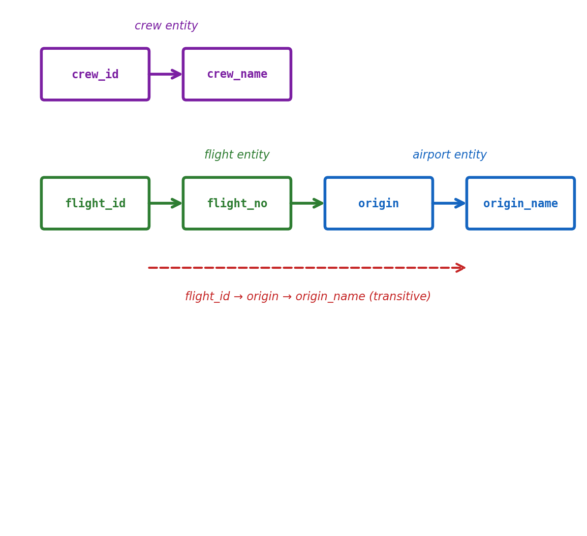
Third Normal Form (3NF)
In 2NF, plus: no non-key column depends on another non-key column. All non-key columns depend directly on the primary key.
Violation — transitive dependency:
flight_id
flight_number
origin
origin_name
origin_tz
7
AA 100
LAX
Los Angeles Intl
America/Los_Angeles
15
DL 47
ATL
Hartsfield-Jackson
America/New_York
23
UA 200
LAX
Los Angeles Intl
America/Los_Angeles
flight_id → origin (direct)
origin → origin_name, origin_tz (direct, but origin is not a key)
flight_id → origin → origin_name (transitive)
The airport name and timezone depend on the origin code, not on the flight. They belong in the airports table, not the flights table.
3NF — remove transitive dependencies:
flights:
flight_id
flight_number
origin
7
AA 100
LAX
15
DL 47
ATL
23
UA 200
LAX
airports:
airport_code
name
timezone
LAX
Los Angeles Intl
America/Los_Angeles
ATL
Hartsfield-Jackson
America/New_York
Airport name stored once. "Los Angeles Intl" no longer duplicated across flights. Updating the name requires changing one row.
The aviation schema from section 02 is already in 3NF. Each table stores attributes that depend on that table’s primary key and nothing else.
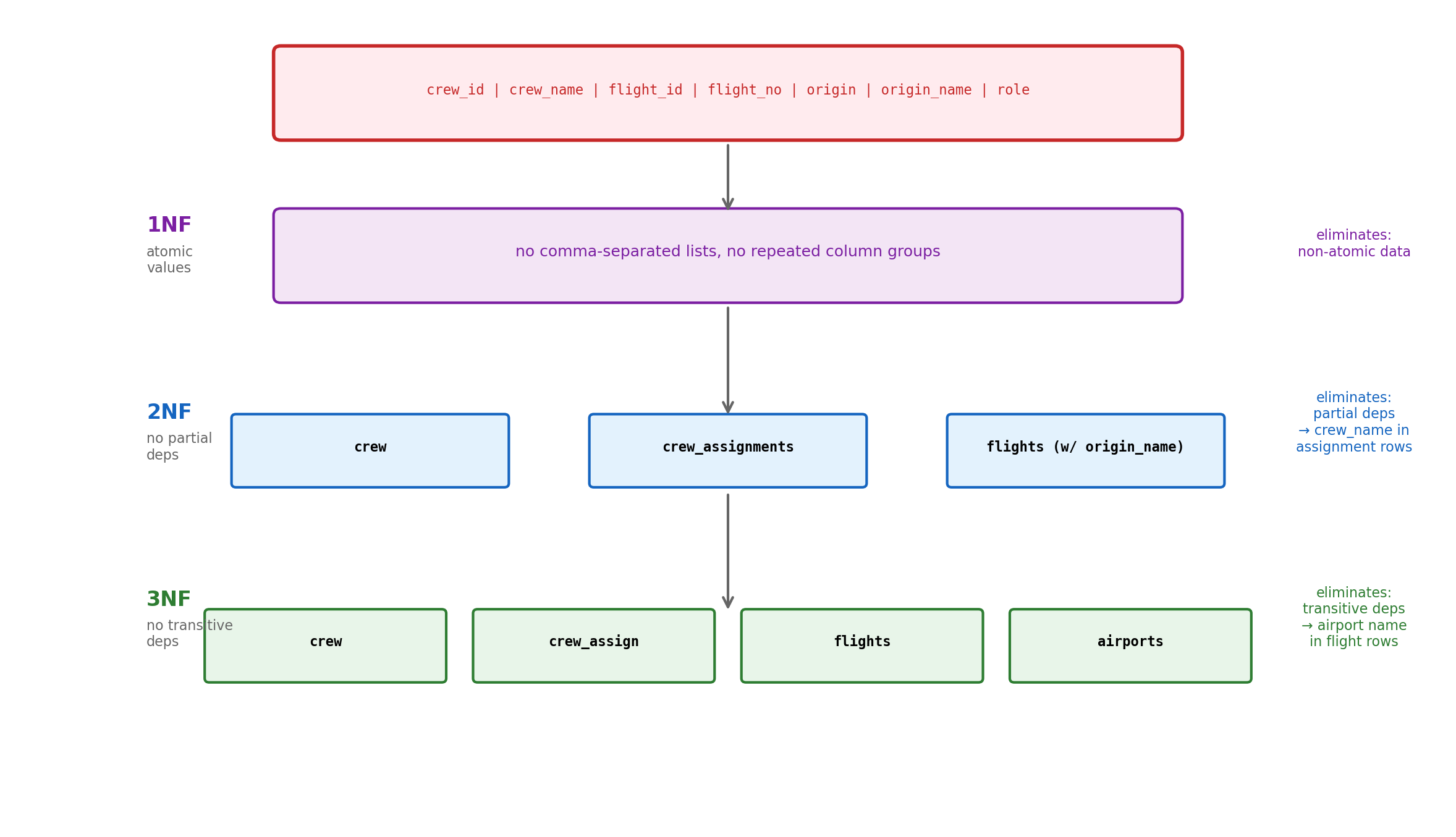
Normalization Progression
Each step eliminates a class of dependency violation. The end state: each fact stored exactly once.
Denormalization as a Deliberate Trade-off
Normalization eliminates redundancy. But normalized data is distributed across tables, and reassembling it requires joins.
Normalized — correct, join-dependent:
SELECT b.booking_id, f.flight_number, a.name AS airportFROM bookings bJOIN flights f ON b.flight_id = f.flight_idJOIN airports a ON f.origin = a.airport_codeWHERE b.passenger_id =42;
Three tables joined. Airport name stored once — always consistent.
Cost: CPU and I/O for the join. Negligible at small scale; measurable at millions of rows with complex join graphs.
One table, no joins, faster reads. But origin_name duplicated in every booking row.
Cost: storage, write complexity, anomaly risk. Updating an airport name means updating every booking row that references it — partial updates produce inconsistency.
Denormalized — faster reads, consistency becomes the application’s responsibility
Denormalization Is the Foundation of NoSQL
NoSQL databases make denormalization a first-class design principle rather than a reluctant optimization.
Relational (normalized):
Schema enforces structure
Joins reassemble related data
Writes are simple (one fact, one place)
Reads may require multiple joins
Horizontal scaling is difficult — joins require data co-location
Any query can combine any tables. Schema evolves by adding tables and relationships. The cost: join complexity at scale.
Document store (denormalized):
Data stored as self-contained documents
Related data embedded within the document
No joins — everything for one request in one read
Writes must update every copy of duplicated data
Horizontal scaling straightforward — documents are independent
Each document contains everything needed to serve a request. The cost: managing redundancy and consistency across documents when the same fact is embedded in thousands of places.
Transactions and Concurrency
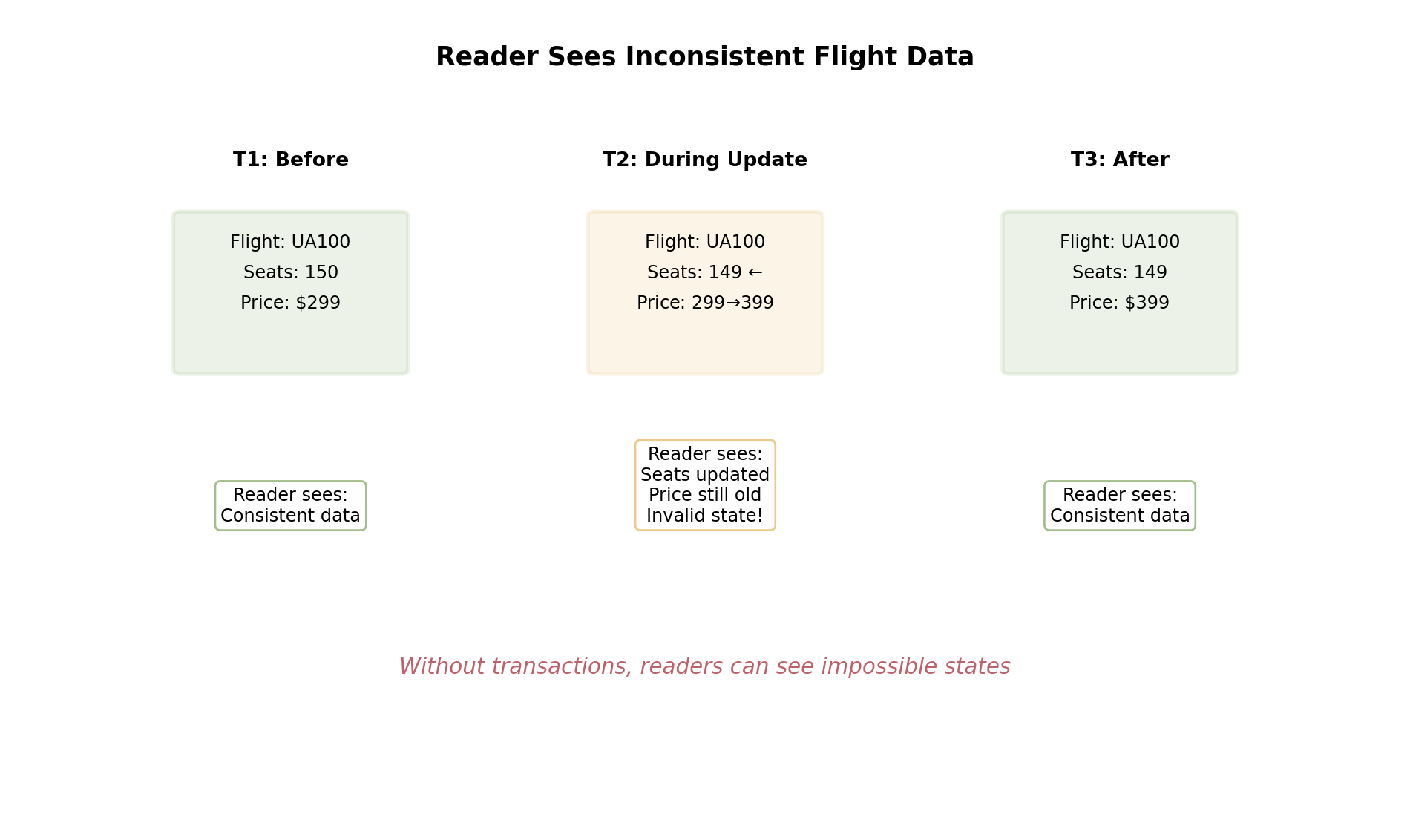
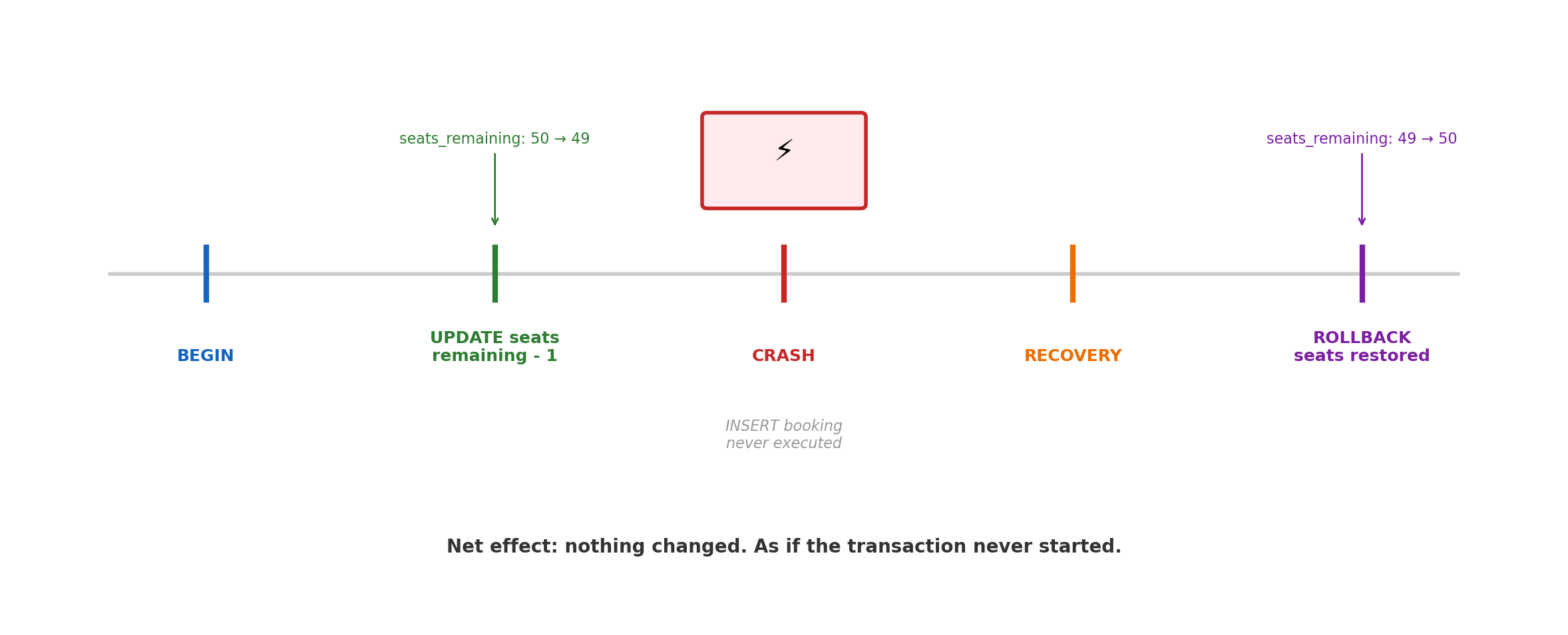
Transactions Group Operations into Atomic Units
A booking requires two writes: decrement the seat count, then insert the booking record. If the second fails, the first must be undone.
Transaction A’s uncommitted changes are invisible to transaction B (at most isolation levels)
Behaves as if transactions ran sequentially
The database achieves this while actually running them concurrently
Durability — committed data survives failures
After COMMIT returns, the data is on stable storage
Write-ahead log (WAL) ensures this: log entry written and fsynced before commit acknowledged
Server loses power one millisecond after COMMIT → data intact on restart
Atomicity Under Failure
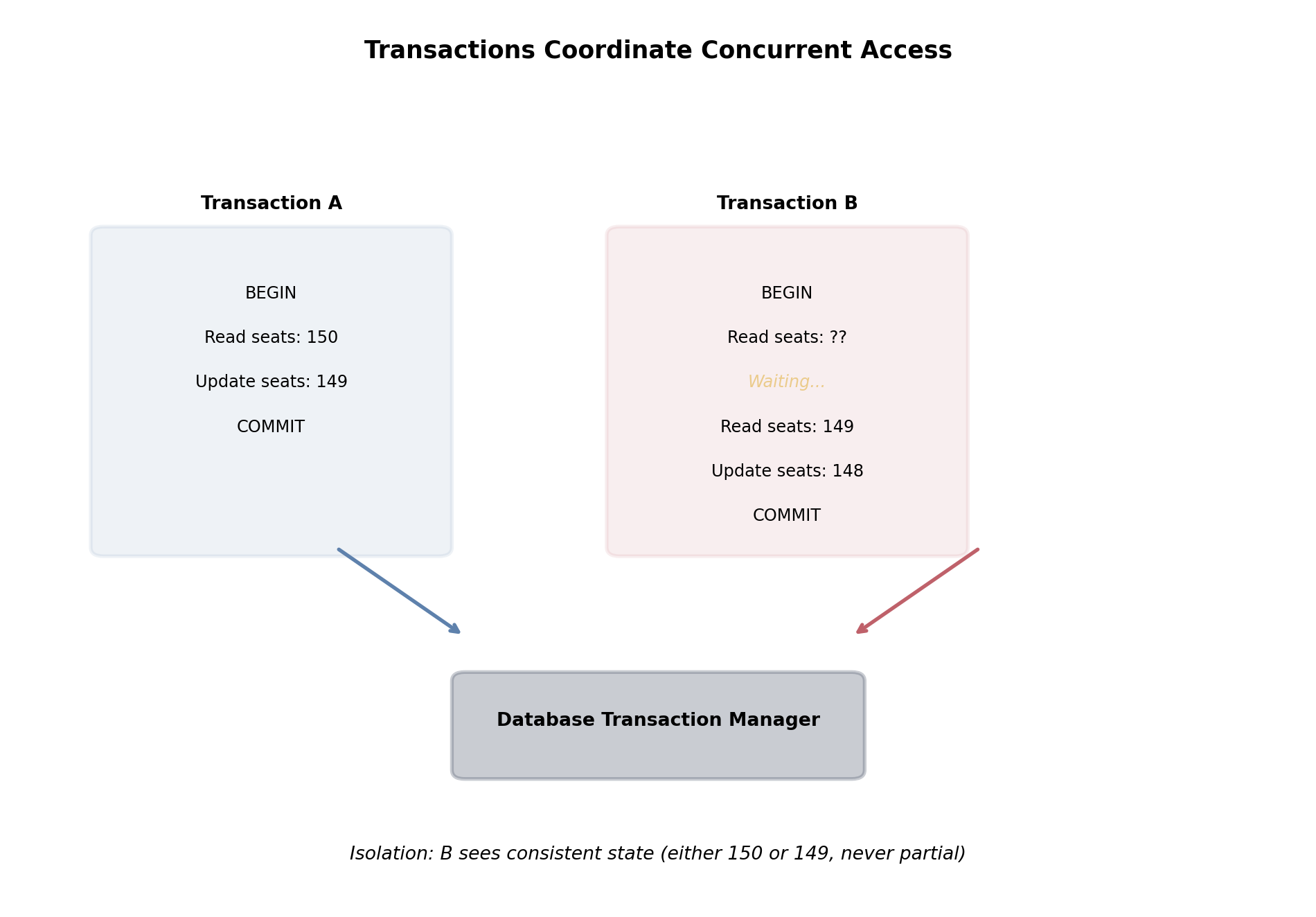
Concurrent Transactions Interleave
Multiple connections execute transactions simultaneously. The database interleaves their operations.
Both transactions read seats_remaining = 1. Both set it to 0. Both commit. The second transaction’s write overwrites the first — a lost update. Neither transaction saw the other’s changes.
Concurrency Anomalies
Dirty read — reading uncommitted data
Tx A updates a seat count but hasn’t committed
Tx B reads the updated (uncommitted) value
Tx A rolls back
Tx B acted on data that never existed
Non-repeatable read — same query, different results
Tx A reads seats_remaining = 5
Tx B updates seats_remaining = 3 and commits
Tx A reads again: seats_remaining = 3
Same query, same transaction, different answer
Phantom read — new rows appear
Tx A queries all bookings for flight 7: 48 rows
Tx B inserts a new booking for flight 7 and commits
Tx A queries again: 49 rows
A row that didn’t exist now appears
Lost update — concurrent write collision
Tx A reads seats_remaining = 1
Tx B reads seats_remaining = 1
Tx A writes seats_remaining = 0, commits
Tx B writes seats_remaining = 0, commits
Two bookings, one seat
Each anomaly represents a different way concurrent transactions can interfere. Isolation levels control which anomalies the database prevents.
Isolation Levels
Four standard levels, each preventing a progressively larger set of anomalies. Higher isolation costs more throughput.
Level
Dirty read
Non-repeatable read
Phantom read
Lost update
READ UNCOMMITTED
possible
possible
possible
possible
READ COMMITTED
prevented
possible
possible
possible
REPEATABLE READ
prevented
prevented
possible
prevented
SERIALIZABLE
prevented
prevented
prevented
prevented
READ COMMITTED (PostgreSQL default)
Each statement sees only data committed before that statement began
Different statements within the same transaction may see different data
Sufficient for most applications
SERIALIZABLE
Behaves as if transactions ran one at a time
Prevents all anomalies
Higher overhead: transactions may fail and need retry
BEGINISOLATIONLEVELSERIALIZABLE;-- operations here see a consistent snapshot-- conflicts cause serialization failureCOMMIT;
Isolation in Practice
The seat booking under READ COMMITTED:
BEGIN;SELECT seats_remaining FROM flightsWHERE flight_id =7; -- returns 1-- another transaction commits here,-- setting seats_remaining to 0UPDATE flightsSET seats_remaining = seats_remaining -1WHERE flight_id =7AND seats_remaining >0;-- rows affected: 0 (condition no longer true)-- application checks: no rows updated → abortROLLBACK;
The WHERE seats_remaining > 0 guard prevents overselling — but only because the UPDATE sees the committed state at the time the UPDATE runs, not the state at the time of the SELECT.
Application-level patterns:
Optimistic concurrency — read, compute, write with a guard condition. If the guard fails, retry.
SELECT … FOR UPDATE — acquire a row lock at read time, preventing concurrent modification until commit.
BEGIN;SELECT seats_remaining FROM flightsWHERE flight_id =7FORUPDATE; -- locks the row-- guaranteed: no other transaction can-- modify this row until we COMMITUPDATE flightsSET seats_remaining = seats_remaining -1WHERE flight_id =7;INSERTINTO bookings ...;COMMIT;
FOR UPDATE trades concurrency for correctness — other transactions reading this row must wait.
Locking: The Mechanism Behind Isolation
Databases enforce isolation through locks — markers that control which transactions can access which data.
Lock granularity:
Row-level — locks one row; other rows in the same table are unaffected
Table-level — locks the entire table; all other access blocked
Row-level is the default for most operations
Lock types:
Shared (read) lock — multiple transactions can hold simultaneously; blocks writers
Exclusive (write) lock — only one holder; blocks all other access to that row
Lock duration:
Held until the transaction ends (COMMIT or ROLLBACK)
Long transactions hold locks longer → more contention
Contention:
Two transactions updating different flights:
Tx A locks flight 7, Tx B locks flight 15
No contention — proceed concurrently
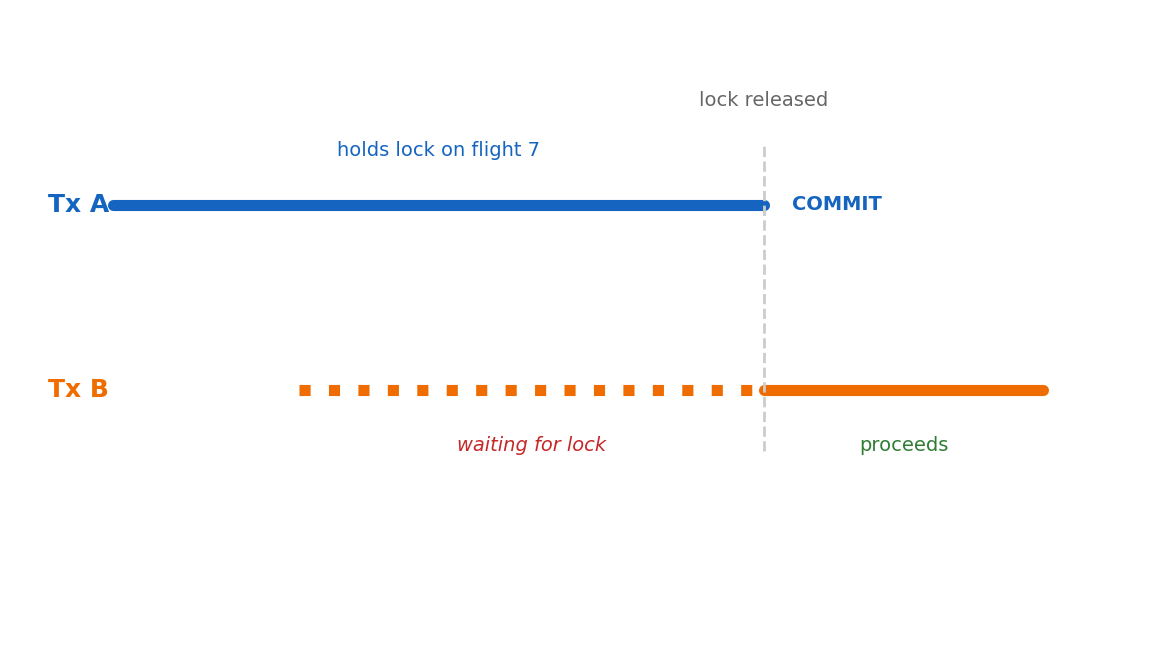
Two transactions updating the same flight:
Tx A locks flight 7
Tx B tries to lock flight 7 → waits
Tx A commits → Tx B proceeds
Lock wait time is the direct cost of isolation. Throughput depends on how often transactions contend for the same rows and how long they hold locks.
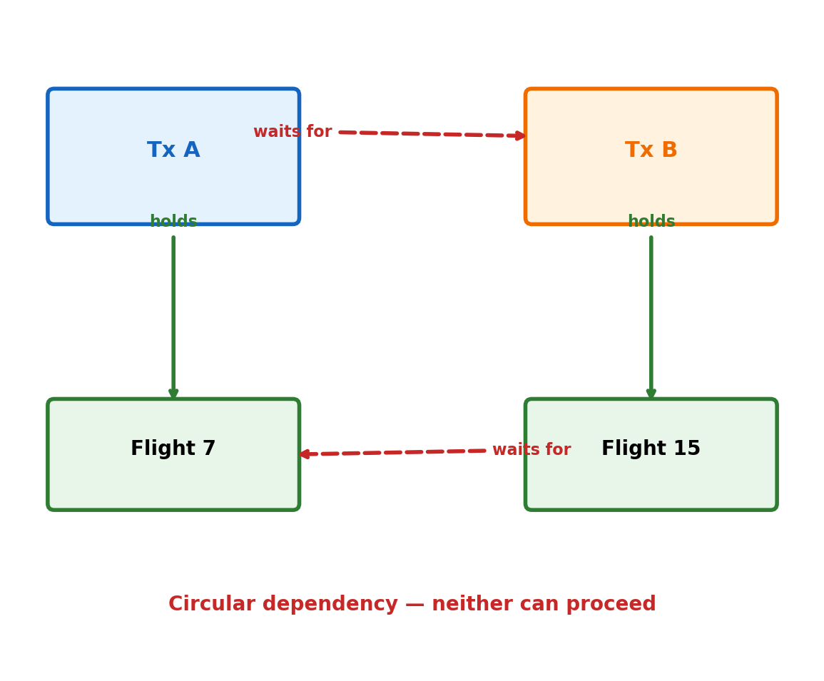
Deadlock
Two transactions, each holding a lock the other needs.
Sequence:
Tx A locks flight 7
Tx B locks flight 15
Tx A requests lock on flight 15 → waits (Tx B holds it)
Tx B requests lock on flight 7 → waits (Tx A holds it)
Neither can proceed. Both will wait forever.
Resolution:
The database detects the cycle (lock dependency graph)
Aborts one transaction (the “victim”)
Victim receives an error; its changes are rolled back
The other transaction proceeds
ERROR: deadlock detected
DETAIL: Process 1234 waits for ShareLock
  on tuple (0,5) of relation "flights";
  blocked by process 5678.
Deadlocks are not bugs — they are an expected consequence of fine-grained locking. Applications must handle the error and retry.
Indexes and Query Performance
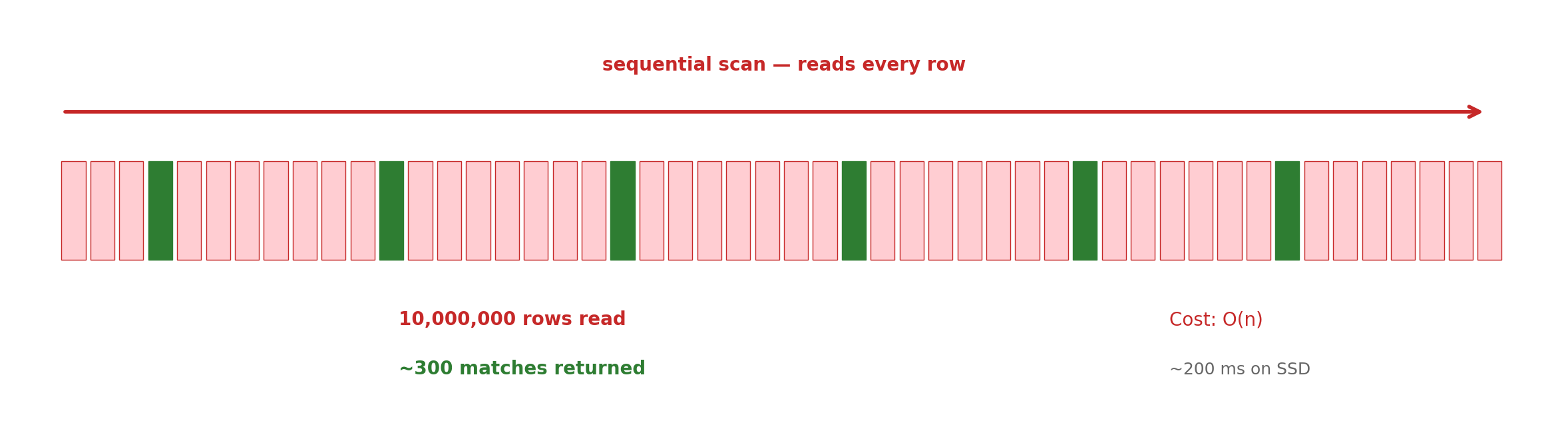
Without an Index, Every Query Scans Every Row
SELECT*FROM flights WHERE origin ='LAX';
No index on origin. The database has no way to locate LAX flights without examining every row.
Sequential scan — the default when no index exists. Cost is proportional to table size, regardless of how many rows actually match. A 10-million-row table takes the same time whether the query matches 3 rows or 3 million.
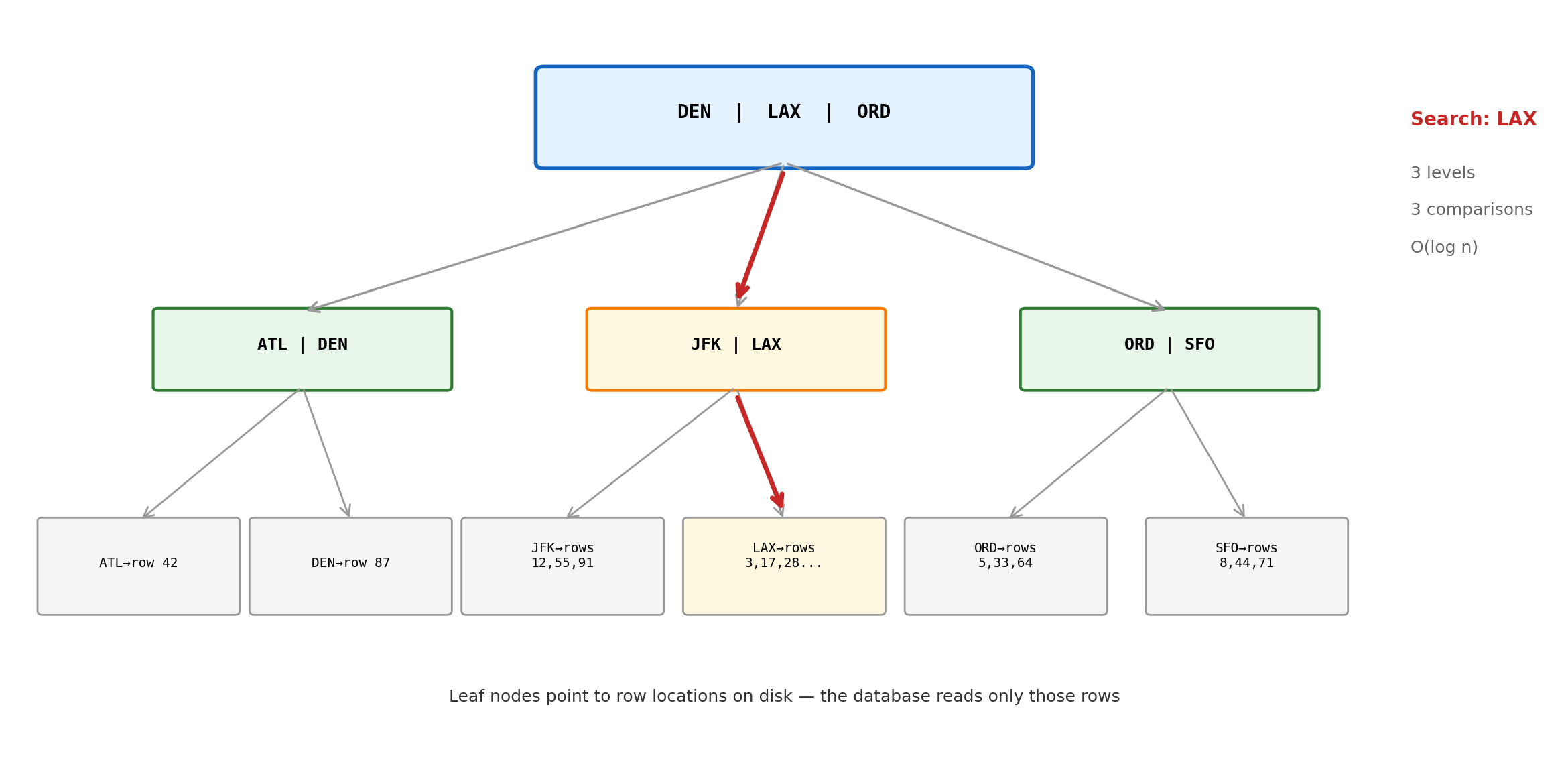
B-Tree: Sorted Lookup Structure
An index is a separate data structure maintained alongside the table. The dominant type is the B-tree — a balanced, sorted tree that maps column values to row locations.
B-tree properties:
Sorted — supports equality (= 'LAX') and range queries (BETWEEN 'LAX' AND 'ORD')
Balanced — all leaf nodes at the same depth; worst-case lookup is O(log n)
10 million rows → ~23 levels (log₂ 10⁷ ≈ 23). Three disk reads instead of ten million.
Maintained automatically — every INSERT, UPDATE, DELETE updates the index
Creating and Using Indexes
CREATEINDEX idx_flights_origin ON flights (origin);
Before the index:
EXPLAIN SELECT * FROM flights WHERE origin=‘LAX’;
Seq Scan on flights Filter: (origin = ‘LAX’) Rows Removed by Filter: 9700 Actual Time: 185.3 ms
After the index:
EXPLAIN SELECT * FROM flights WHERE origin=‘LAX’;
Index Scan using idx_flights_origin Index Cond: (origin = ‘LAX’) Actual Time: 0.8 ms
Same query. Same data. 230x faster.
The optimizer decides whether to use the index.
Selective query (few matches) → index scan
Broad query (most rows match) → seq scan is cheaper
WHERE origin = 'LAX' on a table where 3% of flights are from LAX → index
WHERE seats_remaining > 0 on a table where 95% of flights have seats → seq scan (faster to just read everything)
The decision is automatic. The optimizer maintains statistics on value distributions and chooses the cheapest plan.
CREATE INDEX makes the option available. The optimizer decides when to use it.
The Index Trade-off
Indexes are not free. Every index maintained is a cost paid on every write.
Benefits — read performance:
Equality lookups: O(log n) vs O(n)
Range queries: read a contiguous slice of sorted leaves
ORDER BY on indexed column: already sorted, no sort step
JOIN on indexed column: lookup instead of nested loop
Costs — write performance and storage:
Every INSERT adds an entry to every index on the table
Every UPDATE to an indexed column updates the index
Every DELETE removes an index entry
Each index is a full copy of the indexed columns, sorted differently
A table with 5 indexes: every write does 6 operations (1 table + 5 indexes)
When to index:
Columns in WHERE clauses (filter predicates)
Columns in JOIN conditions (foreign keys)
Columns in ORDER BY (avoid sort step)
High-selectivity columns (few matching rows)
When not to index:
Small tables (seq scan is fast enough)
Columns rarely used in queries
Low-selectivity columns (boolean, status with 3 values)
Write-heavy tables where read performance is less critical
A table with an index on every column pays write overhead and storage cost for each — including indexes no query ever uses. Index selection should be driven by actual query patterns.
Composite Indexes
An index on multiple columns. Column order determines which queries it can serve.
The index sorts by origin first, then by date within each origin.
Queries this index serves:
-- Uses the index (leading column)WHERE origin ='LAX'-- Uses the index (both columns)WHERE origin ='LAX'AND departure_date ='2026-02-12'-- Uses the index (leading column + range)WHERE origin ='LAX'AND departure_date BETWEEN'2026-02-12'AND'2026-02-14'
Queries this index does NOT serve:
-- Cannot use the index (skips leading column)WHERE departure_date ='2026-02-12'
The index is sorted by origin first — without a value for origin, there is no efficient entry point. The database must scan the entire index, no better than a seq scan.
Column order is a design decision driven by query patterns:
(origin, departure_date) — serves “flights from LAX this week”
(departure_date, origin) — serves “all flights today from any airport”
Same columns, different ordering, different queries served efficiently.
Foreign Key Columns Need Indexes
Joins traverse foreign key relationships. Without an index on the FK column, every join becomes a sequential scan of the referenced table.
PostgreSQL does not automatically index foreign key columns.
CREATETABLE bookings ( booking_id SERIAL PRIMARYKEY, flight_id INTEGERREFERENCES flights(flight_id),...);-- flights(flight_id) has a PK index-- bookings(flight_id) has NO index
SELECT*FROM flights fJOIN bookings b ON f.flight_id = b.flight_idWHERE f.origin ='LAX';
For each LAX flight, the database scans every row in bookings to find matches:
Every foreign key column should generally have an index. The write cost of maintaining it is almost always justified by join performance.
MySQL/InnoDB creates FK indexes automatically. PostgreSQL does not — FK index omissions are a frequent source of production performance issues in PostgreSQL deployments.
Relational Architecture at Scale
Fixed Schema: Rigidity as Enforcement
Every row in a table has the same columns. A flight has an origin, a destination, a departure time — regardless of whether the flight is domestic or international, cargo or passenger, scheduled or charter.
All existing flights now have customs_required = NULL — the column exists for every row, including domestic flights where it has no meaning. Charter flights may need columns that scheduled flights do not.
Heterogeneous entities fit awkwardly in fixed schemas. When subtypes have substantially different attributes:
Single table with many nullable columns — sparse, type-dependent NULLs
Multiple tables with shared keys (ISA pattern) — requires joins
Both are valid; both have costs
ALTER TABLE in production is an operational event.
On a table with 100 million rows:
Adding a column with a DEFAULT value rewrites every row (PostgreSQL < 11)
Adding a NOT NULL constraint requires scanning every row to verify
Changing a column type requires rewriting and revalidating every value
These operations acquire locks that block concurrent writes
Schema changes require coordination with application code:
New column the application doesn’t know about → harmless
Removed column the application still references → failure
Schema migration tools (Flyway, Alembic, Django migrations) manage this — versioned scripts applied in sequence, with rollback capability.
Schema Rigidity Is Also Schema Enforcement
The same property that makes schema evolution expensive is what prevents invalid data.
Rigid schema guarantees:
Every flight has an origin — NOT NULL enforced
Every airport code is exactly 3 characters — CHAR(3) enforced
Every booking references a real flight — foreign key enforced
Seat counts never go negative — CHECK constraint enforced
These guarantees hold for every row, every application, every access path. No application can insert a flight without an origin. No background job can set a seat count to -1.
Different fields, no schema violation — because there is no schema.
New fields appear without migration
Nothing prevents "origin": 123 or a missing flight_number
Validation responsibility shifts entirely to application code
Joins Are the Cost of Normalization
Normalized data eliminates redundancy by distributing facts across tables. Retrieving a complete record requires joining those tables back together.
A passenger’s itinerary:
SELECT b.booking_id, f.flight_number, f.departure_time, a_orig.name, a_dest.nameFROM bookings bJOIN flights f ON b.flight_id = f.flight_idJOIN airports a_orig ON f.origin = a_orig.airport_codeJOIN airports a_dest ON f.destination = a_dest.airport_codeWHERE b.passenger_id =42;
Four tables joined. With proper indexes, this runs in milliseconds even at millions of rows.
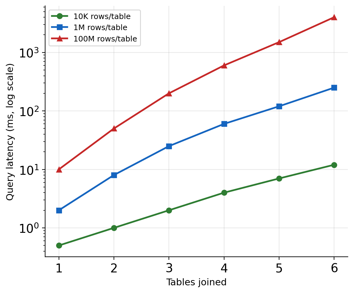
But join cost is not constant. It depends on:
Number of tables joined
Size of each table
Selectivity of join conditions
Available indexes
Whether intermediate results fit in memory
At small scale, joins are negligible. At large scale with many tables, they dominate query time — intermediate result sizes compound across each join.
Some Query Patterns Are Inherently Expensive
Hierarchical data — “all airports reachable within 2 connections from LAX”:
WITH RECURSIVE reachable AS (SELECT destination, 1AS hopsFROM flights WHERE origin ='LAX'UNIONSELECT f.destination, r.hops +1FROM flights fJOIN reachable r ON f.origin = r.destinationWHERE r.hops <2)SELECTDISTINCT destination FROM reachable;
Each recursion level multiplies the working set — three hops from a hub airport can touch millions of rows.
Relational model: relationships via foreign keys, traversal via repeated joins
Graph databases: traversal is a first-class operation with different cost characteristics
Full-text search — “flights with ‘mechanical’ in maintenance notes”:
% prefix prevents index use — sequential scan of every row. PostgreSQL has full-text search extensions (tsvector, tsquery), but these are add-ons, not native relational operations.
Aggregating 100M rows: full table scan regardless of indexes
Row-oriented storage reads entire rows even when only two columns are needed
Columnar storage (Redshift, BigQuery) is purpose-built for this pattern
Relational Databases Are Single-Node Systems
The relational model assumes all data resides on one machine. Cross-table joins, multi-table transactions, and foreign key enforcement all depend on local data access.
Vertical scaling — bigger hardware:
More CPU cores → more concurrent queries
More RAM → larger working set cached, fewer disk reads
Faster storage → lower I/O latency
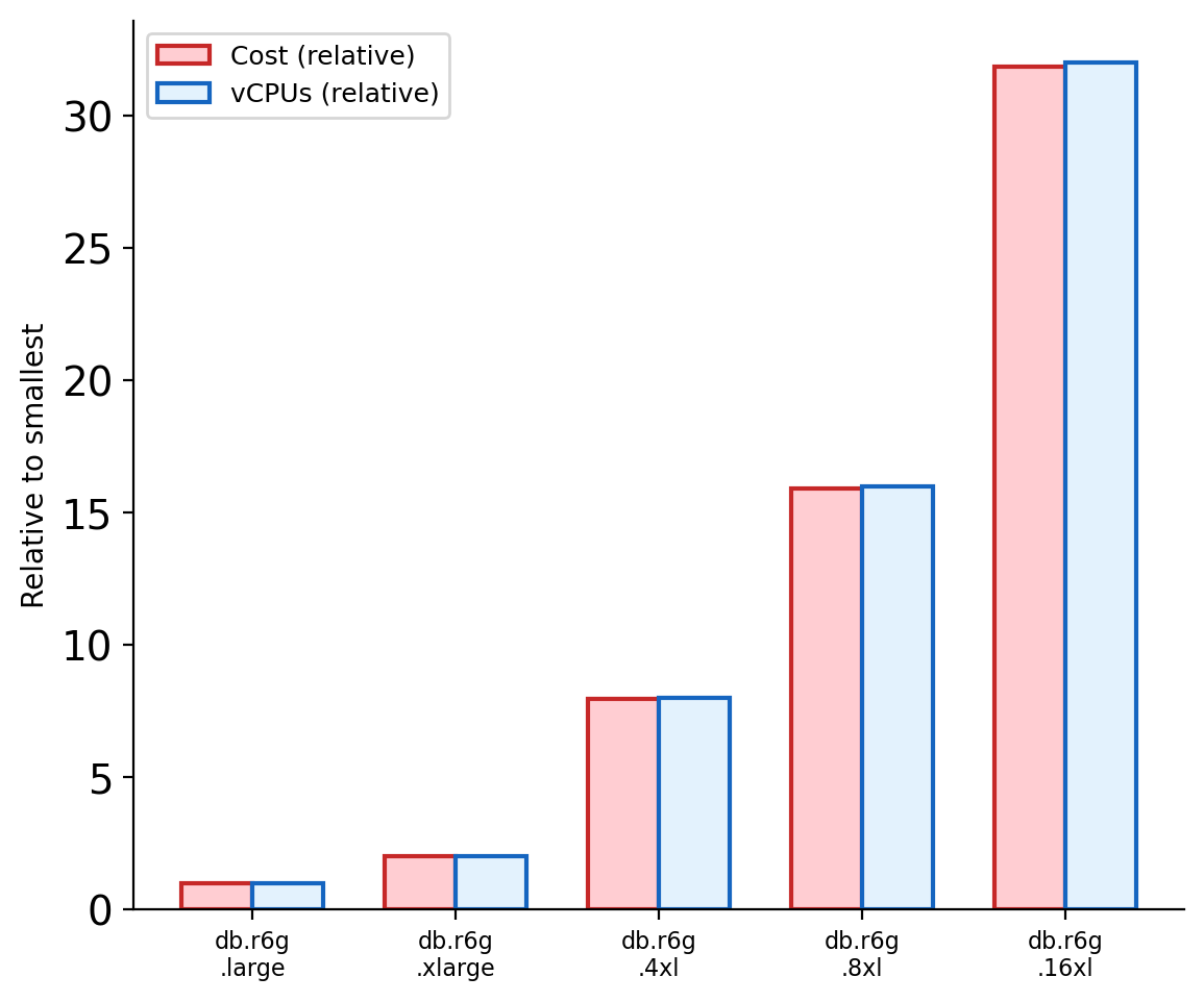
A large managed instance (db.r6g.16xlarge on RDS): 64 vCPUs, 512 GB RAM, provisioned IOPS. Handles millions of rows, thousands of queries per second.
Vertical scaling has a ceiling. The largest available instance is a fixed upper bound. Cost scales faster than capacity — doubling CPU and RAM more than doubles the price.
The 16xl is 32x the cost of the large for 32x the CPU — but real-world throughput does not scale 32x. Lock contention, I/O bottlenecks, and connection overhead erode gains at each tier.
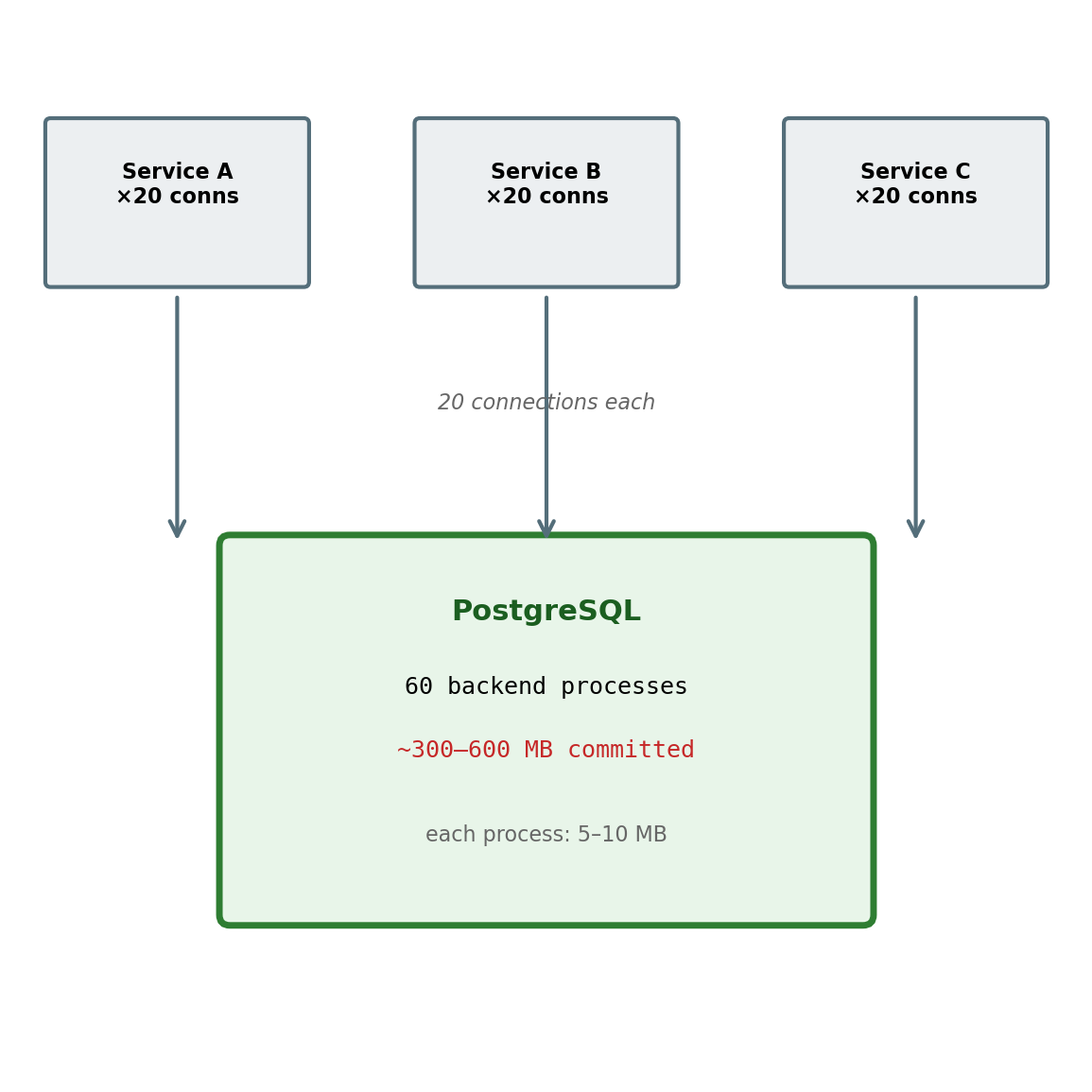
Every Connection Is a Server-Side Process
A database connection is not a lightweight handle. PostgreSQL forks a dedicated backend process for each connection — a separate OS process with its own memory allocation.
Per-connection cost:
~5–10 MB of memory for the backend process
TCP handshake + TLS negotiation + authentication on establishment
A new connection takes ~45 ms to establish over TLS
A simple indexed query takes ~2 ms to execute
For short queries, connection overhead is 95% of total time
Connections accumulate across services.
A db.r6g.xlarge (32 GB RAM) with 5–10 MB per backend has a practical ceiling around 1,000–2,000 concurrent connections before memory pressure degrades query performance for every client.
20 application containers × 20 connections = 400 from one service
Three services sharing the database = 1,200 connections
The limit is reached without any single service behaving unreasonably
Connection Pools Amortize Establishment Cost
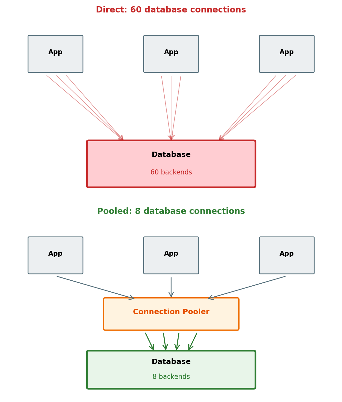
A connection pool maintains a set of open connections and lends them to application threads on demand. The connection is returned after use, not closed — avoiding repeated setup overhead.
Application-side pool — each application instance manages its own pool (HikariCP, SQLAlchemy create_engine(pool_size=...), node-postgres Pool).
Connection reuse: 0.1 ms from pool vs 45 ms to establish
But total database connections = instances × pool size
50 containers × pool of 10 = 500 database connections
Does not solve the aggregate connection count problem at high instance counts
External connection pooler — a proxy between application and database (PgBouncer, RDS Proxy). Many application connections map to fewer database connections.
Multiplexes queries: application “connection” is mapped to a real backend only for the duration of a query or transaction
Required for serverless compute (Lambda) where thousands of short-lived invocations each open a connection
RDS Proxy is the managed AWS equivalent — sits in front of an RDS instance, handles pooling and failover
Pool sizing:
Pool too small → requests queue for a connection; tail latency spikes under load
Pool too large → database memory exhausted; all queries degrade
Starting point: connections = (2 × CPU cores) + spindles for the database host, divided across clients
Horizontal Scaling Breaks Relational Guarantees
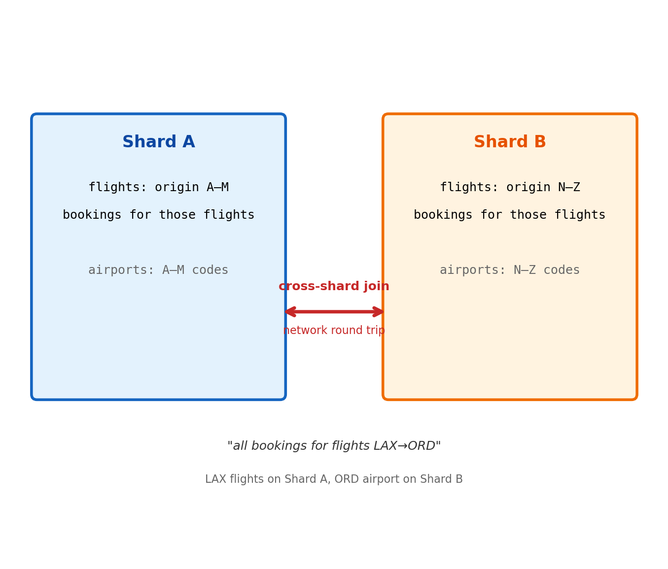
Distributing data across multiple machines (sharding) removes the single-node ceiling — but also removes the assumptions the relational model depends on.
What sharding breaks:
Joins across shards — flights on Shard A, airports on Shard B. Join requires network round trip; data must be shipped between machines.
Cross-shard transactions — require distributed coordination (two-phase commit). Slower, more failure modes, not universally supported.
Foreign key enforcement — Shard A cannot verify a FK references a row on Shard B without querying Shard B on every write.
Global uniqueness — ensuring a unique booking_id when inserts happen on any shard is a distributed consensus problem.
All four are consequences of data locality. The relational model’s guarantees assume all data is locally accessible.
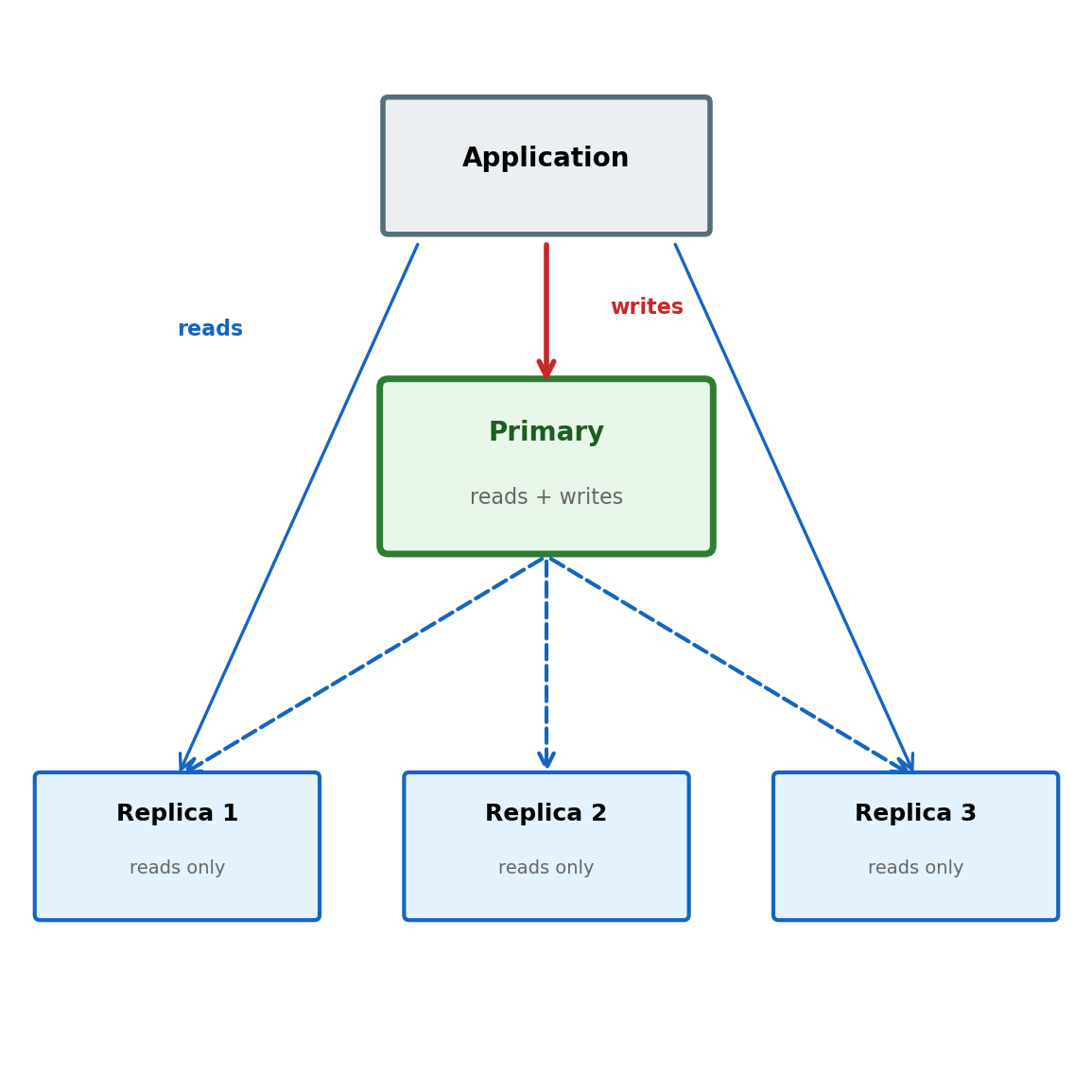
Read Replicas: Partial Horizontal Scaling
Read replicas scale reads while preserving relational guarantees.
A single primary handles all writes
One or more replicas receive a copy of every write (asynchronously)
Read traffic distributed across replicas
Joins, foreign keys, transactions all work — each replica has a complete copy
Scales:
Read throughput — proportional to replica count
Analytical workload isolation — queries on replicas, not the primary
Geographic read latency — replica per region
Does not scale:
Write throughput — single primary, all writes
Storage — every replica holds the full dataset
Write latency — bounded by primary hardware
Replication lag — replicas receive writes asynchronously, typically milliseconds to seconds behind the primary. A write followed by an immediate read from a replica may not see its own write — a common source of confusing application behavior.
The CAP Trade-off in Distributed Systems
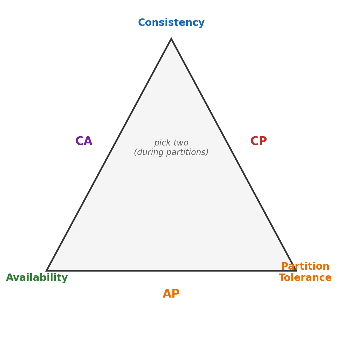
When a system runs on multiple machines connected by a network, three properties are in tension.
Consistency — every read returns the most recent write. All nodes see the same data at the same time.
Availability — every request receives a response, even if some nodes are unreachable.
Partition tolerance — the system continues operating when network links between nodes fail.
Network partitions are inevitable in distributed systems — hardware fails, switches drop packets, links go down. A system must tolerate partitions, leaving a choice between consistency and availability during a partition:
CP (consistency + partition tolerance) — relational databases. If the primary loses contact with a replica, writes are rejected or the replica stops serving reads. Stale data is prevented; some requests fail.
AP (availability + partition tolerance) — e.g., some document stores. Writes accepted on both sides of a partition, reconciled later. Every request gets a response; reads may return stale data.
The choice depends on the domain. A banking system cannot tolerate stale balances. A content feed can tolerate a post appearing seconds late.
Relational Trade-offs Are Design Choices
What the relational model provides:
Schema enforcement — invalid data rejected at write time, consistent for all clients
Declarative querying — any combination of tables can be joined, filtered, aggregated
Transactional guarantees — atomicity, isolation, durability enforced by the database
Referential integrity — relationships between tables are maintained automatically
Normalization — each fact stored once, no update anomalies
The application does not validate types, enforce relationships, coordinate concurrent access, or manage crash recovery. The database handles these — which simplifies application code but constrains the system’s architecture.
Join dependency — normalized data requires reassembly; cost grows with volume and complexity
Single-node architecture — vertical scaling has a ceiling; horizontal scaling breaks guarantees
Consistency priority — availability sacrificed during network partitions
Each cost is the direct consequence of a guarantee. Systems that offer flexible schemas, join-free reads, or horizontal scaling achieve them by shifting the corresponding responsibility to application code.