NoSQL and Distributed Databases

-- Natural queries for uniform data
SELECT * FROM bookings
WHERE passenger_id = 1234;

SELECT f.* FROM flights f
WHERE departure_airport = 'LAX'
  AND arrival_airport = 'JFK';

When data and queries match structure, relational wins

Schema Rigidity When Data Varies

Add special services to passengers:

Wheelchair assistance
Meal preferences (vegetarian, gluten-free, kosher)
Pet carrier
Unaccompanied minor
Medical oxygen
Extra legroom request

Relational approach 1: Add columns

ALTER TABLE passengers ADD COLUMN wheelchair BOOLEAN;
ALTER TABLE passengers ADD COLUMN meal_pref VARCHAR(50);
ALTER TABLE passengers ADD COLUMN pet_carrier BOOLEAN;
-- ...12 more columns

Problem: Most passengers have mostly NULLs (90% of cells)

Relational approach 2: Services table

CREATE TABLE passenger_services (
  passenger_id INT,
  service_key VARCHAR(50),
  service_value TEXT
);

Problem: Loses type safety, querying awkward

-- Find passengers needing wheelchair
SELECT DISTINCT passenger_id
FROM passenger_services
WHERE service_key = 'wheelchair'
  AND service_value = 'true';

-- Complex: wheelchair AND vegetarian
SELECT ps1.passenger_id
FROM passenger_services ps1
JOIN passenger_services ps2
  ON ps1.passenger_id = ps2.passenger_id
WHERE ps1.service_key = 'wheelchair'
  AND ps2.service_key = 'meal_pref'
  AND ps2.service_value = 'vegetarian';

Neither approach feels natural — data has variable structure per entity

Approach 1 storage example:

passenger_id	name	wheelchair	meal	pet	oxygen	…
1	Alice	NULL	NULL	NULL	NULL	…
2	Bob	NULL	vegan	NULL	NULL	…
3	Carol	true	NULL	NULL	NULL	…

With 10,000 passengers: 10,000 rows × 15 service columns = 150,000 cells, ~135,000 NULL values

Variable Schema Problem Generalizes

E-commerce products:

Books:

ISBN: VARCHAR(13)
author: VARCHAR(100)
pages: INT
publisher: VARCHAR(100)

Electronics:

voltage: INT
warranty_months: INT
power_watts: INT
battery_type: VARCHAR(50)

Clothing:

size: VARCHAR(10)
material: VARCHAR(100)
care_instructions: TEXT
fit_type: VARCHAR(50)

Relational solution?

Single products table with 50+ columns, mostly NULL
product_attributes table (key-value pairs)
Separate tables per category (breaks product queries)

IoT sensor data:

Temperature sensors:

celsius: FLOAT
calibration_date: DATE

Motion sensors:

x_accel: FLOAT
y_accel: FLOAT
z_accel: FLOAT
sensitivity: INT

Camera sensors:

image_url: VARCHAR(500)
resolution_width: INT
resolution_height: INT
fps: INT
codec: VARCHAR(20)

Pattern: Entity type is uniform (product, sensor), but attributes vary within type

Relational model assumes: All entities of same type have same attributes

Reality: Many domains have heterogeneous attributes

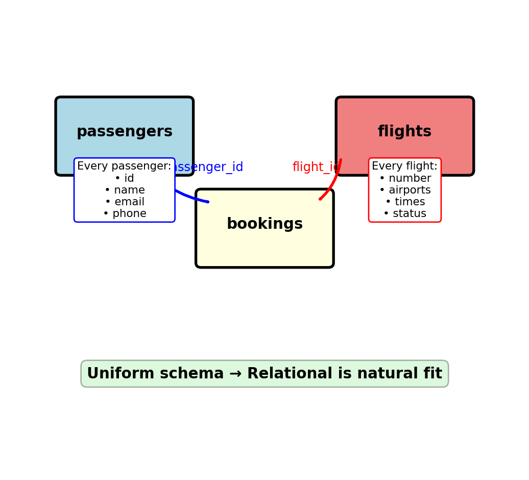
Nested Data Requires JOIN Operations for Reassembly

Application code thinks in objects:

# Natural object access
booking.passenger.frequent_flyer_number
booking.flight.departure_airport
booking.flight.aircraft.model

SQL requires JOIN to reassemble:

SELECT b.*, p.*, f.*, a.*
FROM bookings b
  JOIN passengers p ON b.passenger_id = p.passenger_id
  JOIN flights f ON b.flight_id = f.flight_id
  JOIN aircraft a ON f.aircraft_id = a.aircraft_id
WHERE b.booking_id = 12345;

Computational cost:

Each JOIN: O(n log n) at best with indexes
Three JOINs for three-level nesting
Deeply nested structures → multiple JOINs

Worse: Comments on posts on forums

-- Get comment with post and forum context
SELECT c.*, p.*, f.*
FROM comments c
  JOIN posts p ON c.post_id = p.post_id
  JOIN forums f ON p.forum_id = f.forum_id;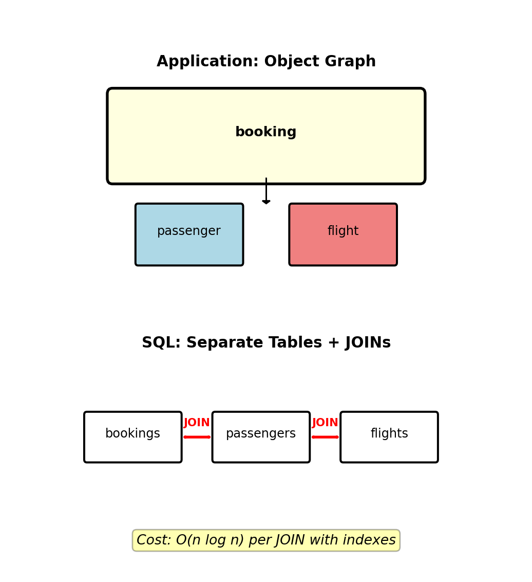

Impedance mismatch: Object hierarchy vs tabular relations

Every nested access = JOIN operation

Impedance Mismatch - Serialization Round-Trips

Impedance mismatch: Application code operates on object graphs, databases store flat tables. Moving data between these representations requires expensive translation.

Loading a passenger with 3 bookings and flight details:

# ORM loading pattern (N+1 query problem)
passenger = session.query(Passenger).get(123)  # 1 query
for booking in passenger.bookings:              # 1 query
    flight = booking.flight                     # 3 queries
    aircraft = flight.aircraft                  # 3 queries
# Total: 8 queries

Eager loading with JOINs:

SELECT p.*, b.*, f.*, a.*
FROM passengers p
  LEFT JOIN bookings b ON p.passenger_id = b.passenger_id
  LEFT JOIN flights f ON b.flight_id = f.flight_id
  LEFT JOIN aircraft a ON f.aircraft_id = a.aircraft_id
WHERE p.passenger_id = 123;

Result: Duplicated passenger data × 3 rows (one per booking)

Alternative: Serialize entire object as JSON

-- Store object as JSON blob
ALTER TABLE passengers ADD COLUMN data JSONB;

Problem: Lose query capability, indexing, constraints

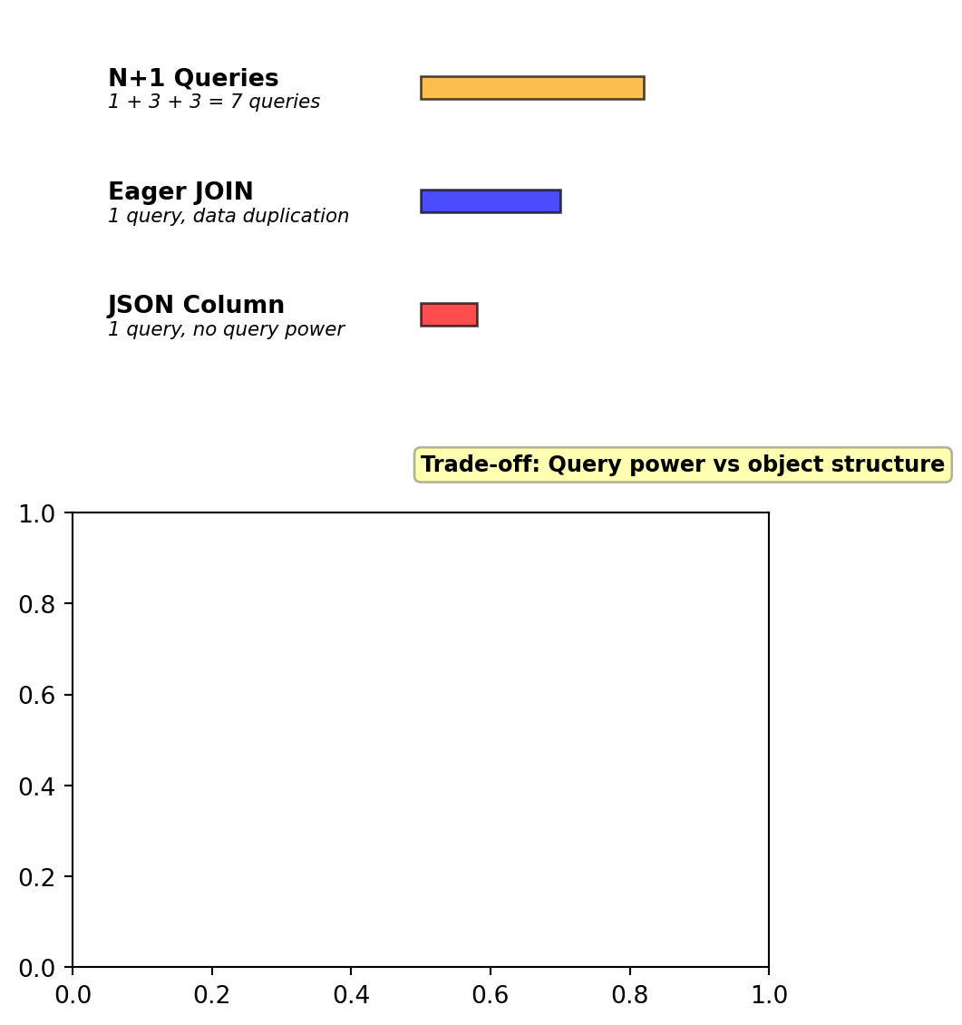
Load time for 1 passenger + 3 bookings:

N+1 Queries: 45ms (7 roundtrips)
Eager JOIN: 12ms (data duplication across rows)
JSON Column: 3ms (no additional queries, but limited query power)

Each approach has serious drawbacks

Query Patterns That Fight Relational Structure

Relational optimized for:

Get entity by ID: O(1) with primary key
Filter on indexed columns: O(log n)
JOIN related tables: O(n log n)

Problematic patterns:

1. Path queries:

-- Flights connecting through exactly 2 hubs
SELECT f1.flight_number, f2.flight_number, f3.flight_number
FROM flights f1
  JOIN flights f2 ON f1.arrival_airport = f2.departure_airport
  JOIN flights f3 ON f2.arrival_airport = f3.departure_airport
WHERE f1.departure_airport = 'LAX'
  AND f3.arrival_airport = 'LHR'
  AND f1.arrival_airport NOT IN ('LAX', 'LHR')
  AND f2.arrival_airport NOT IN ('LAX', 'LHR');

Self-JOINs explode with path length

2. Sparse attribute filters:

-- Passengers with (gluten-free OR wheelchair) AND pet
SELECT DISTINCT ps1.passenger_id
FROM passenger_services ps1
WHERE ps1.passenger_id IN (
    SELECT passenger_id FROM passenger_services
    WHERE (service_key = 'meal' AND service_value = 'gluten-free')
       OR (service_key = 'wheelchair' AND service_value = 'true')
  )
  AND ps1.passenger_id IN (
    SELECT passenger_id FROM passenger_services
    WHERE service_key = 'pet_carrier' AND service_value = 'true'
  );

3. Full-text search:

-- Passengers whose names contain substring
SELECT * FROM passengers
WHERE first_name LIKE '%john%'
   OR last_name LIKE '%john%';

Cannot use B-tree index, requires full table scan

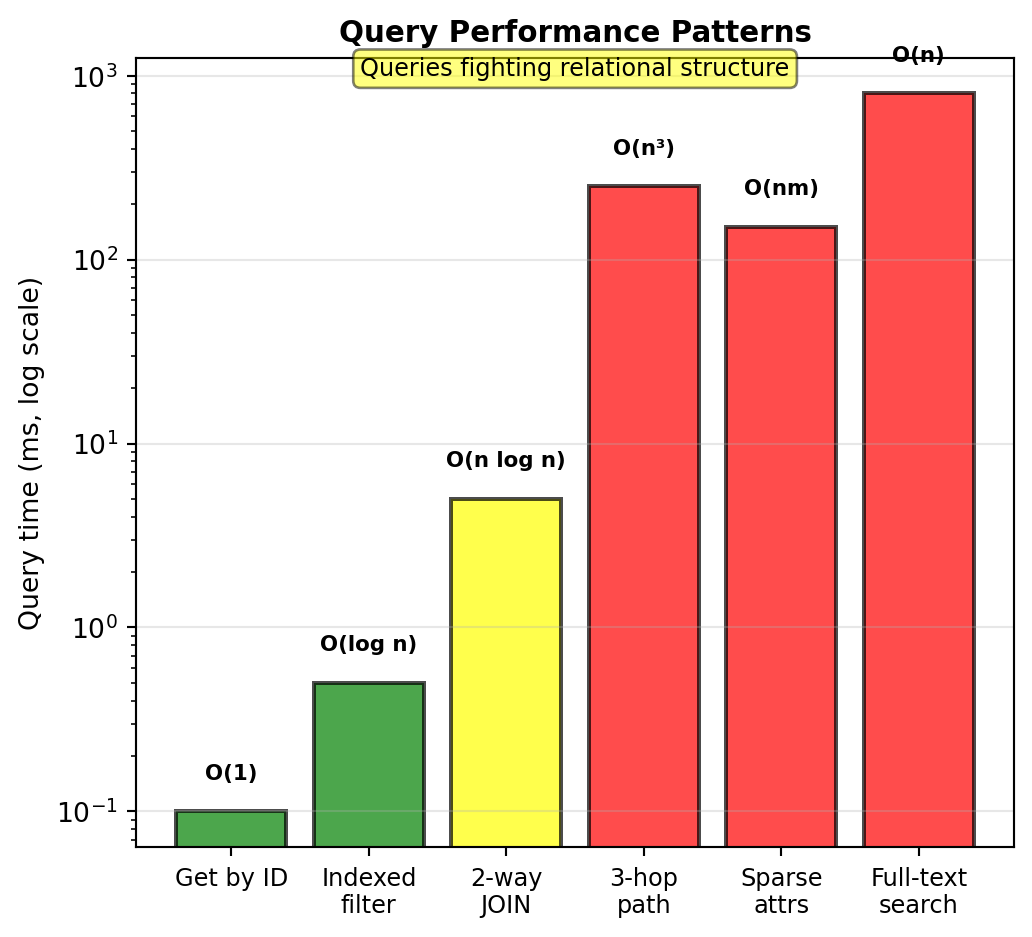
These work but feel forced, require complex queries, or full table scans

Social Connection Queries in Relational Models

Schema:

CREATE TABLE users (
  id SERIAL PRIMARY KEY,
  name VARCHAR(100),
  city VARCHAR(50)
);

CREATE TABLE connections (
  user_id INT REFERENCES users(id),
  friend_id INT REFERENCES users(id),
  PRIMARY KEY (user_id, friend_id)
);

Query: “Friends of friends who live in Boston”

SELECT DISTINCT u.*
FROM connections c1
  JOIN connections c2 ON c1.friend_id = c2.user_id
  JOIN users u ON c2.friend_id = u.id
WHERE c1.user_id = 123
  AND u.city = 'Boston'
  AND c2.friend_id != 123;

Cost: 2 self-JOINs, O(n²) join complexity

3-hop traversal (friends-of-friends-of-friends)?

3 self-JOINs, O(n³) complexity
Each additional hop: another JOIN, exponential growth

Arbitrary depth?

Requires recursive CTEs (complex, poorly optimized)

Recursive CTEs:

WITH RECURSIVE paths AS (
  SELECT user_id, friend_id, 1 AS depth
  FROM connections
  WHERE user_id = 123
  UNION ALL
  SELECT p.user_id, c.friend_id, p.depth + 1
  FROM paths p
  JOIN connections c ON p.friend_id = c.user_id
  WHERE p.depth < 5
)
SELECT DISTINCT friend_id FROM paths;

Complex, performance unpredictable

JSON Columns Provide Flexibility But Limits Query Power

PostgreSQL JSONB, MySQL JSON type:

ALTER TABLE passengers ADD COLUMN services JSONB;

-- Store variable data as JSON
INSERT INTO passengers (id, name, email, services)
VALUES (1, 'Alice', 'alice@example.com',
  '{"wheelchair": true, "meal": "vegetarian"}');

INSERT INTO passengers (2, 'Bob', 'bob@example.com',
  '{"meal": "gluten-free", "pet_carrier": true, "extra_legroom": true}');

Querying JSON data:

-- PostgreSQL JSONB operators
SELECT * FROM passengers
WHERE services->>'wheelchair' = 'true';

SELECT * FROM passengers
WHERE services ? 'meal'
  AND services->>'meal' = 'vegetarian';

Problems:

Query optimization: Cannot use B-tree indexes on nested paths efficiently
Partial indexes help but don’t solve fundamental issue

CREATE INDEX idx_wheelchair
ON passengers ((services->>'wheelchair'))
WHERE services->>'wheelchair' IS NOT NULL;

Type constraints lost: Everything is text in JSON
No foreign key relationships inside JSON

Performance comparison:

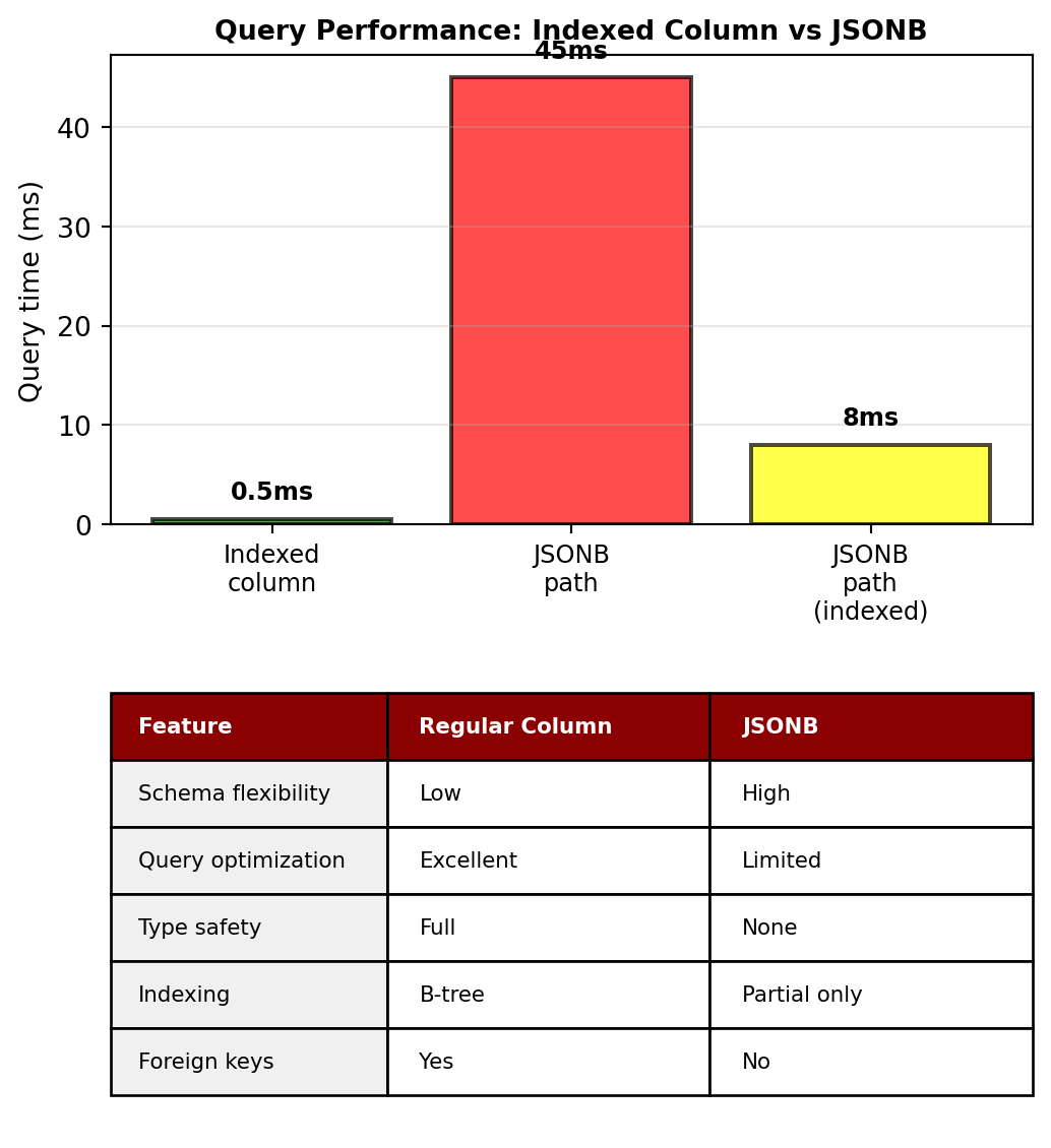
Result: Relational overhead without relational benefits for nested data

Better solutions exist when data is fundamentally non-tabular

Sparse Data and NULL Proliferation

Add event tracking to flights:

ALTER TABLE flights ADD COLUMN delay_reason VARCHAR(100);
ALTER TABLE flights ADD COLUMN delay_minutes INT;
ALTER TABLE flights ADD COLUMN diverted_airport CHAR(3);
ALTER TABLE flights ADD COLUMN emergency_landing BOOLEAN;
ALTER TABLE flights ADD COLUMN diversion_reason TEXT;
ALTER TABLE flights ADD COLUMN emergency_type VARCHAR(50);
ALTER TABLE flights ADD COLUMN emergency_services BOOLEAN;
ALTER TABLE flights ADD COLUMN passenger_medical BOOLEAN;
-- ...15 more event-specific columns

Most flights: NULL for all special event fields

flight_id	delay_reason	diverted	emergency	…
1001	NULL	NULL	NULL	…
1002	NULL	NULL	NULL	…
1003	weather	NULL	NULL	…
1004	NULL	NULL	NULL	…

With 1M flights, 20 event columns:

20M total cells
19M NULLs (95%)
Storage waste: Implementation-dependent, but significant

Semantic ambiguity:

NULL = unknown?
NULL = does not apply?
NULL = not recorded?

Querying sparse data is awkward:

-- Find flights with delays NOT due to weather
SELECT * FROM flights
WHERE delay_reason IS NOT NULL
  AND delay_reason != 'weather';

-- Flights with ANY special event
SELECT * FROM flights
WHERE delay_reason IS NOT NULL
   OR diverted_airport IS NOT NULL
   OR emergency_landing IS NOT NULL
   OR passenger_medical IS NOT NULL
   -- ...15 more conditions

Sparse attributes common in:

Event tracking
Optional features
User preferences
Sensor readings
Medical records

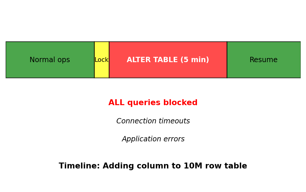
Schema Evolution Under Load

Need to add column to flights table with 10M rows:

ALTER TABLE flights ADD COLUMN delay_minutes INTEGER;

PostgreSQL behavior:

Acquires ACCESS EXCLUSIVE lock
Blocks ALL reads and writes during operation
On large tables: Minutes of downtime
Application connections timeout and fail

Timing for different table sizes:

Rows	ALTER TABLE time	Downtime
10K	~1 second	Acceptable
100K	~10 seconds	Problematic
1M	~30 seconds	Unacceptable
10M	~5 minutes	Critical

Zero-downtime migration requires shadow table (complexity: high, time: hours)

Application-level workaround (complex):

Create shadow table with new schema
Implement dual-write to both tables
Backfill old data to new table
Switch application to new table
Drop old table

Error-prone:

Maintaining data consistency during migration
Coordinating application deployments
Rollback strategy if issues arise

Relational Remains Correct for Structured Data

Flight operations data FITS relational well:

Uniform schema:

Every flight has same structure
Every booking follows same pattern
Every passenger has consistent attributes

Clear relationships:

Foreign keys model real entities
Referential integrity enforced by database
JOIN operations match conceptual relationships

Transaction requirements:

Booking seat → decrease inventory atomically
Payment + confirmation must succeed together
ACID properties critical for correctness

Known queries:

Predictable access patterns
Standard reporting needs
Queries match table structure

-- These queries are natural and efficient
SELECT COUNT(*) FROM bookings WHERE flight_id = 1234;

SELECT f.*, COUNT(b.booking_id) as passenger_count
FROM flights f
LEFT JOIN bookings b ON f.flight_id = b.flight_id
GROUP BY f.flight_id;

BEGIN TRANSACTION;
  INSERT INTO bookings (passenger_id, flight_id, seat)
  VALUES (123, 456, '12A');
  UPDATE flights SET available_seats = available_seats - 1
  WHERE flight_id = 456;
COMMIT;

If your data looks like this, relational is the correct choice

When relational is correct:

Uniform schema per entity type
Relationships map to foreign keys
ACID transactions required
Queries match table structure
Data integrity constraints needed

When to consider alternatives:

Variable attributes per entity
Deep object hierarchies
Sparse/optional attributes
Graph traversal queries
Frequent schema changes

Match data structure to model — not every problem needs NoSQL

Query Patterns Define Data Model

Relational Normalizes, NoSQL Denormalizes

Relational modeling:

Normalize to 3NF, eliminate redundancy
Single source of truth for each fact
JOIN to assemble complete views

NoSQL modeling:

Start with queries, store data for read patterns
Redundancy acceptable for query performance
Trade storage and update complexity for read simplicity

Example: Flight booking confirmation email

Relational approach: JOIN 5 tables

SELECT b.booking_reference, p.name, p.email,
       f.flight_number, f.scheduled_departure,
       d.name AS departure_city,
       a.name AS arrival_city,
       ac.model AS aircraft_type
FROM bookings b
  JOIN passengers p ON b.passenger_id = p.passenger_id
  JOIN flights f ON b.flight_id = f.flight_id
  JOIN airports d ON f.departure_airport = d.airport_code
  JOIN airports a ON f.arrival_airport = a.airport_code
  JOIN aircraft ac ON f.aircraft_id = ac.aircraft_id
WHERE b.booking_id = 12345;

NoSQL approach: Store complete confirmation in booking document

{
  "booking_id": 12345,
  "booking_reference": "ABC123",
  "passenger": {
    "name": "Alice Chen",
    "email": "alice@example.com"
  },
  "flight": {
    "number": "UA123",
    "departure": "2025-02-15T08:30:00Z",
    "departure_city": "Los Angeles",
    "arrival_city": "New York",
    "aircraft": "Boeing 737"
  }
}

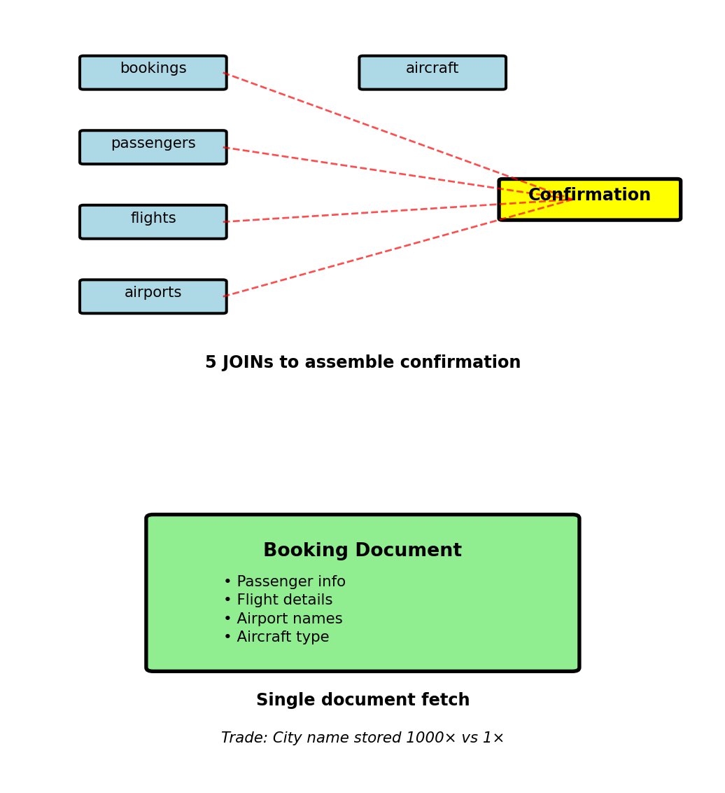
Update cost: User name changes → update in 1000 places vs 1 place

When acceptable: Reads >> Writes (confirmation viewed 100× more than user changes name)

Access Pattern - Flight Status Display

Requirement: Airport display showing flight status

Refreshes every 30 seconds
Shows next 2 hours of departures
100 displays at LAX

Query: “All departures from LAX in next 2 hours”

Data needed:

Flight number, gate, status
Destination city name (not just code)
Aircraft type
Departure time

Relational approach:

SELECT f.flight_number, f.gate, f.status,
       f.scheduled_departure,
       a.model AS aircraft_type,
       ap.name AS destination_city
FROM flights f
  JOIN aircraft a ON f.aircraft_id = a.aircraft_id
  JOIN airports ap ON f.arrival_airport = ap.airport_code
WHERE f.departure_airport = 'LAX'
  AND f.scheduled_departure BETWEEN NOW()
      AND NOW() + INTERVAL '2 hours';

Frequency analysis:

100 displays × 120 queries/hour = 12,000 queries/hour
Schedule changes: ~5 updates/hour
Read:Write ratio = 2400:1

NoSQL approach: Denormalize for display query

{
  "flight_id": 1234,
  "flight_number": "UA123",
  "departure_airport": "LAX",
  "arrival_airport": "JFK",
  "destination_city": "New York",  // Duplicated
  "aircraft_model": "Boeing 737",   // Duplicated
  "gate": "B12",
  "status": "On Time",
  "scheduled_departure": "2025-02-15T14:30:00Z"
}

Single query, no joins:

db.flights.find({
  departure_airport: "LAX",
  scheduled_departure: {
    $gte: new Date(),
    $lte: new Date(Date.now() + 2*60*60*1000)
  }
})

Read:Write ratio 2400:1 justifies denormalization

Aircraft model duplicated in every flight using that aircraft

City name duplicated in every flight to that destination

Updates rare, reads constant

Embedding - Passenger Special Services

Earlier Problem: Variable passenger services

Wheelchair assistance
Meal preferences
Pet carrier
Varying per passenger

Document approach: Embed services as nested object

{
  "passenger_id": 123,
  "name": "Alice Chen",
  "email": "alice@example.com",
  "phone": "+1-555-0123",
  "services": {
    "wheelchair": true,
    "meal": "vegetarian",
    "pet_carrier": true,
    "seat_preference": "aisle",
    "medical_oxygen": false
  },
  "frequent_flyer": {
    "number": "FF123456",
    "tier": "Gold",
    "miles": 85000
  }
}

Why embed:

Accessed together in primary query pattern
Small size (<1KB total)
No independent existence
Services have no meaning without passenger context

Single document fetch gets everything

No NULL columns for passengers without services

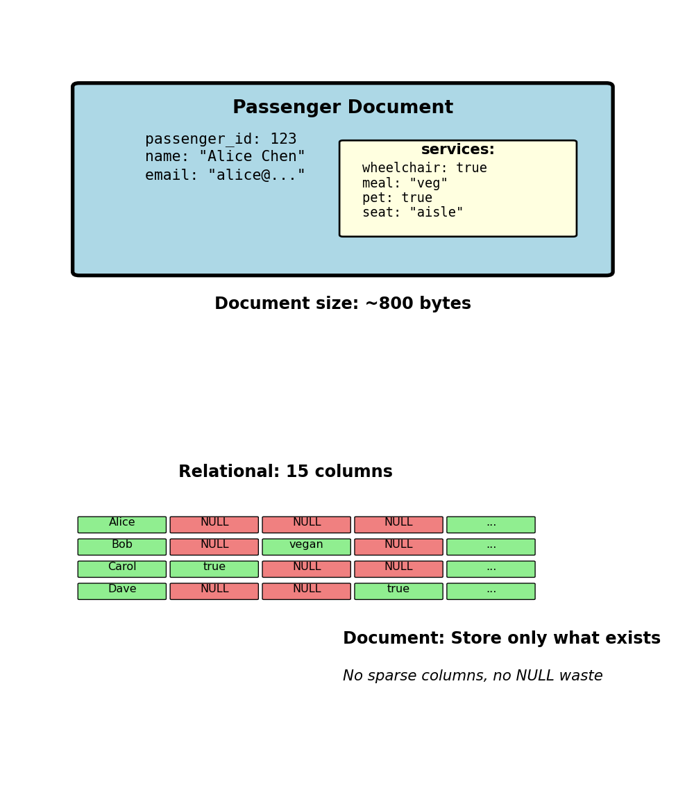
Store only what exists, no wasted NULL storage

Referencing - Flight Bookings

Flight with 200 bookings - cannot embed all:

Size problem:

200 bookings × 1KB each = 200KB
MongoDB limit: 16MB
DynamoDB limit: 400KB
Approaching limits with just bookings

Access problem:

Fetching flight details does not need all bookings
Display shows “seats available”, not passenger list
Loading 200KB when 1KB needed

Update problem:

Every new booking rewrites entire flight document
Concurrent booking updates conflict
Document-level locking affects all bookings

Solution: Reference pattern

// Flight document (small, frequently accessed)
{
  "flight_id": 456,
  "flight_number": "UA123",
  "departure_airport": "LAX",
  "arrival_airport": "JFK",
  "scheduled_departure": "2025-02-15T14:30:00Z",
  "seats_available": 12,
  "total_seats": 180
}

// Booking document (separate collection)
{
  "booking_id": 789,
  "flight_id": 456,  // Reference to flight
  "passenger_id": 123,
  "seat": "12A",
  "booking_time": "2025-01-15T10:30:00Z"
}

Query patterns:

Get flight details:

db.flights.findOne({flight_id: 456})
// Returns 1KB document

Get bookings for flight:

db.bookings.find({flight_id: 456})
// Returns cursor to 200 documents

Add new booking:

// Two operations (in transaction if supported)
db.bookings.insert({...})
db.flights.update(
  {flight_id: 456},
  {$inc: {seats_available: -1}}
)

Trade-off:

Embedded: 200 KB document (grows with bookings)
Referenced: 1 KB flight + 1 KB per booking (separate queries)
Document size limit: 16 MB (MongoDB)

Like foreign keys, but application-enforced (not database engine!)

Sensor Data at Scale - Distribution Patterns

Scenario: IoT temperature sensor network

100,000 sensors
1 reading per minute per sensor
5 years retention required

Data volume:

100K sensors × 60 readings/hour = 6M readings/hour
144M readings/day
52.6B readings/year
5 years = 263B readings

Cannot fit on single server:

263B readings × 50 bytes/reading = 13TB
Query latency unacceptable on 13TB
Write throughput: 1,667 writes/second continuous

Read patterns:

Recent readings for one sensor (95% of queries)
- “Sensor 42000 last 24 hours”
All readings for sensor in time range (4%)
- “Sensor 42000 January 2025”
Average across all sensors (1%)
- “Average temperature now”

Distribution required: 13TB cannot fit on single server

Partition strategy determines query efficiency:

Primary pattern: Single sensor queries (99%)
Rare pattern: Cross-sensor aggregation (1%)

Sensor Data - Partition by Sensor ID

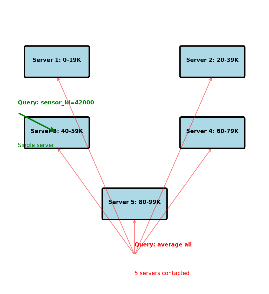
Partition strategy: All data for sensor_id on same server

Physical layout across 5 servers:

Server 1: sensor_id 0-19,999 (20K sensors)
Server 2: sensor_id 20,000-39,999
Server 3: sensor_id 40,000-59,999
Server 4: sensor_id 60,000-79,999
Server 5: sensor_id 80,000-99,999

Each server stores:

sensor_id | timestamp           | temperature
----------|--------------------|-----------
40000     | 2025-01-15 00:00  | 21.0
40000     | 2025-01-15 00:01  | 21.1
40000     | 2025-01-15 00:02  | 21.2
...
40001     | 2025-01-15 00:00  | 19.5

Query 1: “Sensor 42000, last 24 hours”

Hash(42000) → Server 3
Route query to single server
Single server processes query
Fast: O(1) routing, O(log n) within server

Query 2: “Average temperature all sensors”

Must contact all 5 servers
Each computes local average
Coordinator aggregates results
Slow: 5× network calls

Performance:

Single sensor query: ~5ms
All sensors query: ~50ms (parallel) + aggregation

Partition key determines query efficiency

Sensor Data - Row Structure Optimized for Queries

Query requirement: Readings with metadata

Location where sensor installed
Sensor type and calibration info
Building/floor information

Relational approach (bad for distributed):

-- Metadata on central server
CREATE TABLE sensors (
  sensor_id INT PRIMARY KEY,
  location VARCHAR(100),
  building VARCHAR(50),
  sensor_type VARCHAR(20)
);

-- Readings partitioned across 5 servers
CREATE TABLE readings (
  sensor_id INT,
  timestamp TIMESTAMP,
  temperature FLOAT,
  FOREIGN KEY (sensor_id) REFERENCES sensors
);

Query needs metadata:

Fetch metadata from central server
Fetch readings from data server
Join in application = 2 network round-trips

Denormalized approach:

{
  "sensor_id": 42000,
  "timestamp": "2025-01-15T10:30:00Z",
  "temperature": 22.5,
  "location": "Building A, Floor 3, Room 301",  // Duplicated
  "sensor_type": "indoor_temp",                  // Duplicated
  "building": "Building A"                       // Duplicated
}

Storage trade-off:

+40 bytes per reading (metadata)
263B readings × 40 bytes = 10.5TB extra
Total: 23.5TB vs 13TB

Query performance:

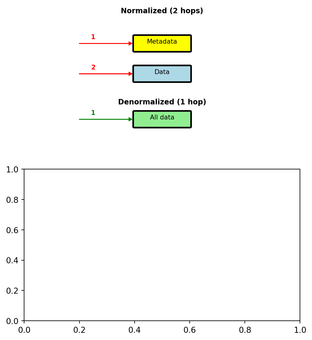
Query performance:

Normalized: 25ms (2 server roundtrips)
Denormalized: 5ms (single server)

Update frequency:

Sensor location changes: ~1 per month
Temperature readings: 100K per minute

Denormalization justified by read:write ratio

Sensor Data - Compound Sort Key for Time Queries

Data on Server 3 (sensor_id 40,000-59,999):

Primary: Partition by sensor_id
Secondary: Sort by timestamp within partition

Physical layout on disk:

Partition: sensor_id=40000
--------------------------
timestamp            | temp
2025-01-15 00:00:00 | 21.0
2025-01-15 00:01:00 | 21.1
2025-01-15 00:02:00 | 21.2
...
2025-01-15 23:59:00 | 20.8

Partition: sensor_id=40001
--------------------------
timestamp            | temp
2025-01-15 00:00:00 | 19.5
2025-01-15 00:01:00 | 19.6
...

Query: “sensor_id=40000 between 10:00 and 12:00”

Hash(40000) → locate partition
Binary search to find 10:00:00
Sequential scan until 12:00:00
Return ~120 readings

Efficient: O(log n) + O(k) where k = result size

Cannot efficiently query: “All sensors at 10:00”

Would scan all 20,000 partitions on this server
Then contact other 4 servers
Query pattern not supported by layout

Sort order within partition provides O(log n) range queries

Multiple Access Patterns Require Multiple Tables

Two different access patterns:

Pattern 1: Recent readings by sensor

“Get sensor 42000 for last 24 hours”
Need: Partition by sensor_id, sort by timestamp

Pattern 2: All sensors at specific time

“Get all sensors at 10:00-11:00”
Need: Partition by timestamp, sort by sensor_id

Same data, stored twice:

-- Table 1: Optimized for sensor queries
CREATE TABLE readings_by_sensor (
  sensor_id INT,        -- Partition key
  timestamp TIMESTAMP,  -- Sort key
  temperature FLOAT,
  location TEXT,
  PRIMARY KEY (sensor_id, timestamp)
);

-- Table 2: Optimized for time queries
CREATE TABLE readings_by_time (
  time_bucket INT,      -- Partition key (hour)
  sensor_id INT,        -- Sort key
  temperature FLOAT,
  location TEXT,
  PRIMARY KEY (time_bucket, sensor_id)
);

Write path: Application writes to both tables

Read path: Query router chooses table based on pattern

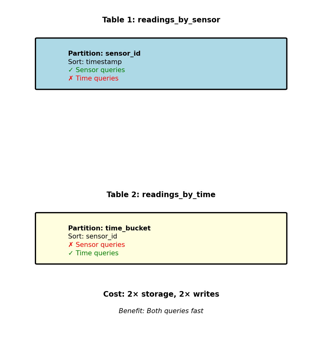
Cannot optimize single table for both patterns

Trade storage and write complexity for query performance

NoSQL Data Modeling Anti-Pattern - Relational Thinking

Anti-pattern: Normalize sensor data

// Sensors collection (metadata)
{
  "sensor_id": 42000,
  "location": "Building A, Floor 3",
  "sensor_type": "indoor_temp",
  "calibration_date": "2024-01-15"
}

// Readings collection (data)
{
  "reading_id": 999999,
  "sensor_id": 42000,  // Reference
  "timestamp": "2025-01-15T10:30:00Z",
  "temperature": 22.5
}

Query to display dashboard (100 recent readings):

Fetch 100 readings from readings collection
Extract unique sensor_ids
Fetch sensor metadata for each unique sensor
Join in application

Problem:

100 readings from 20 sensors = 21 queries
Network latency: 20ms × 21 = 420ms
Dashboard refresh every second? Impossible

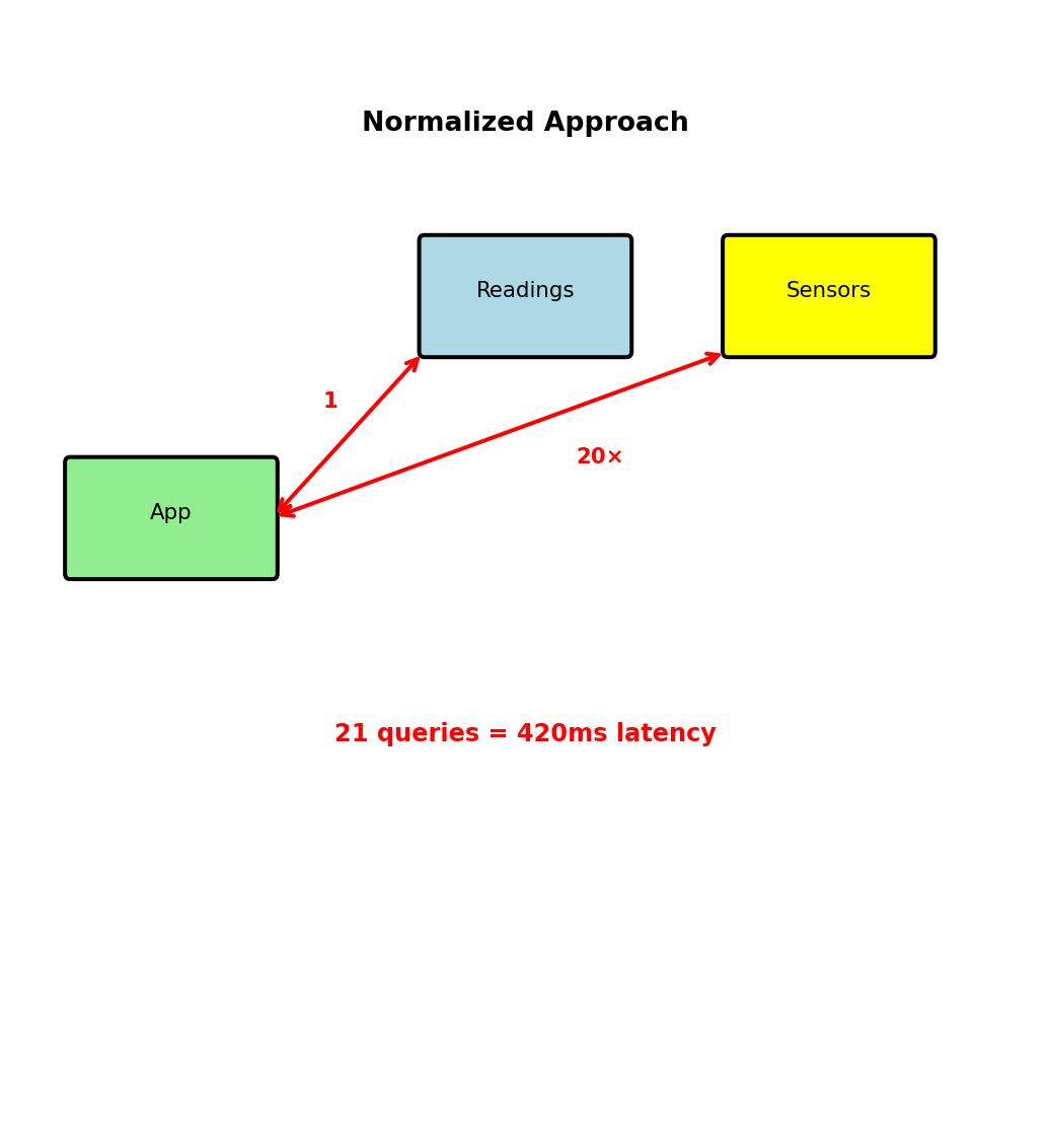
Correct approach: Denormalize

Store location with every reading
Single query returns everything
Latency: 20ms total (21× faster)

Relational normalization creates N+1 query problem

When Denormalization Breaks - Update Anomalies

Scenario: Sensor relocated (Building A → Building B)

With denormalization, location stored in:

1,440 readings per day (every minute)
43,200 readings per month
518,400 readings per year

Update options:

Option 1: Update all historical records

db.readings.updateMany(
  {sensor_id: 42000},
  {$set: {location: "Building B, Floor 2"}}
)

518,400 documents updated
Takes minutes on distributed system
Blocks other operations
Historical data now incorrect

Option 2: Update going forward only

Historical: “Building A”
Current: “Building B”
Query results inconsistent
Acceptable for time-series

Option 3: Versioned metadata

{
  "sensor_id": 42000,
  "timestamp": "2025-01-15T10:30:00Z",
  "temperature": 22.5,
  "metadata_version": 3  // Reference version
}

More complex queries, additional lookup

When denormalization acceptable:

Read:Write > 100:1
Updates rare (monthly)
Eventual consistency OK
Historical accuracy not critical

When to avoid:

Frequent updates (prices change hourly)
Strong consistency required (inventory)
Write-heavy workloads
Regulatory accuracy requirements

Trade-off: Read performance vs update complexity

Scaling and Distribution Trade-offs

Single Node Capacity Limits

PostgreSQL practical limits on single node:

Connections: 10,000 concurrent (connection overhead)
Queries: 100,000 queries/sec (CPU bound)
Storage: ~2TB practical limit (vacuum, index maintenance)
Single point of failure

Real production at scale:

Netflix streaming service:

230M subscribers
1% concurrent = 2.3M active users
10 requests/sec per user = 23M requests/sec
Single node handles: 100K requests/sec
Required: 230+ database nodes minimum

Reddit (2023):

14TB PostgreSQL database
Schema migrations: 6 hours of downtime
Read replicas: 50+ to handle read load

Single-machine limits: Cannot fit internet-scale workloads on one node

Single node limits:

Resource	Limit	Bottleneck
Connections	10K	Memory overhead
Queries/sec	100K	CPU cores
Storage	2TB	Vacuum time
Write throughput	50K/sec	Disk I/O

Capacity mismatch:

Example workload (social media):

100M users
5% active concurrently = 5M
5 queries/user/sec = 25M queries/sec

Single PostgreSQL node: 100K queries/sec

Gap: 250× capacity needed

Cannot be solved with bigger hardware — must distribute across multiple nodes

Vertical vs Horizontal Scaling Economics

Vertical scaling = bigger machine:

AWS RDS pricing (2024):

128GB RAM: $1,380/month → $10.78/GB
1TB RAM: $11,040/month → $10.78/GB
4TB RAM: $38,880/month → $9.72/GB
8TB RAM: $77,760/month → $9.72/GB

Capacity scaling:

10× data requires 10× RAM
10× queries requires 10× CPU
But: 10× cost gets 10× capacity (best case)

Problems with vertical:

Single point of failure
Limited by hardware (8TB RAM max)
Downtime for upgrades
Cannot add capacity gradually

At Reddit’s 14TB:

No single machine available
Must distribute anyway

Horizontal scaling = more machines:

10 nodes × 128GB RAM:

Capacity: 1.28TB total
Cost: 10 × $1,380 = $13,800/month
Redundancy: Lose 1 node, still operational
Incremental: Add nodes as needed

Comparison for 1TB capacity:

Approach	Configuration	Cost	Redundancy
Vertical	1 × 1TB	$11,040	None
Horizontal	10 × 128GB	$13,800	9 nodes survive failure

Horizontal advantages:

Linear cost scaling
Built-in redundancy
No single point of failure
Add capacity without downtime

Trade-off: Horizontal requires distributing data and coordinating across nodes

Partitioning Splits Data Across Nodes

Partition = subset of data assigned to one node

Example: 10M users, 10 nodes

Each node stores 1M users
Query routes to node containing requested data

Two partitioning strategies:

Hash-based partitioning:

node = hash(user_id) % num_nodes

hash("alice") = 0x7a3f → Node 7
hash("bob") = 0x2c91 → Node 2
hash("carol") = 0x9e5d → Node 9

Characteristics:

Even distribution (no hotspots)
Random assignment
Range queries scan all nodes

Range-based partitioning:

A-B → Node 1
C-E → Node 2
F-J → Node 3
...
Z → Node 10

"alice" → Node 1
"bob" → Node 1
"carol" → Node 2

Characteristics:

Range scans stay on few nodes
Risk: Hotspots if data skewed

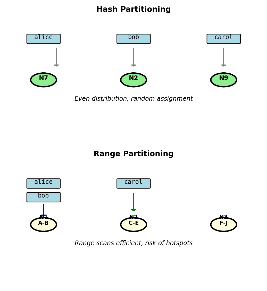
Trade-off: Even load vs efficient range queries

Partition Key Determines Data Location and Query Routing

Partition key = attribute used to determine node assignment

Example: E-commerce orders table

Option 1: Partition by user_id

-- Efficient: Single node
SELECT * FROM orders WHERE user_id = 123;
→ hash(123) = Node 4 → Query Node 4 only

-- Expensive: All nodes
SELECT * FROM orders WHERE order_date = '2024-10-07';
→ Must query all 10 nodes, merge results

Option 2: Partition by order_date

-- Efficient: Single node
SELECT * FROM orders WHERE order_date = '2024-10-07';
→ '2024-10-07' in range for Node 3 → Query Node 3 only

-- Expensive: All nodes
SELECT * FROM orders WHERE user_id = 123;
→ Date unknown, must query all 10 nodes

Partition key choice optimizes one access pattern at expense of others

Cost of wrong choice:

Single-node query: 10ms latency
Cross-partition query: 10 nodes × 10ms = 100ms latency
Plus: Network coordination overhead

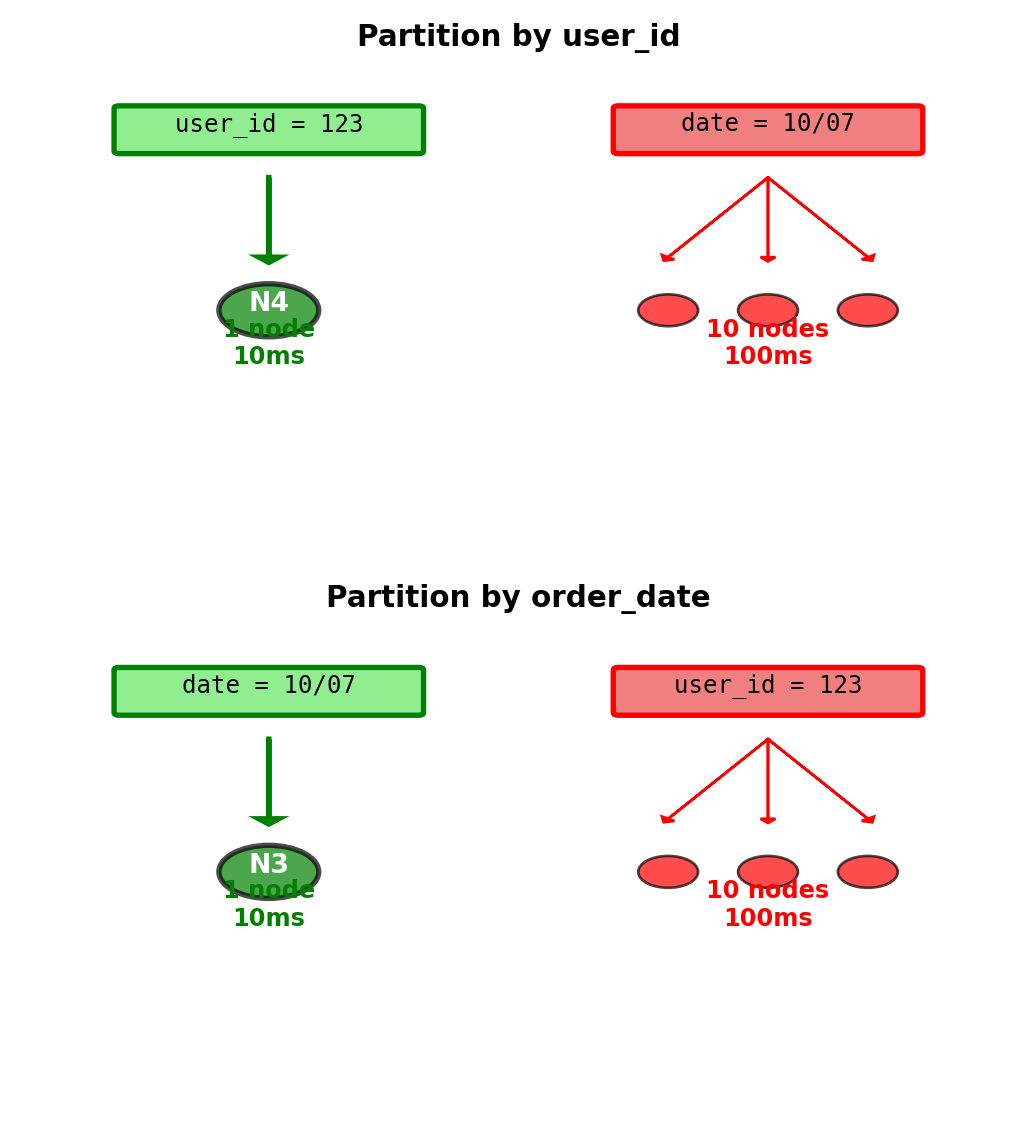
Partition key choice determines which queries are efficient

Replication Provides Redundancy

Replication = store multiple copies of data on different nodes

Why replicate:

1. Fault tolerance:

Disk failure: 0.5% annual failure rate
With 100 nodes: Expect 1 failure every 2 months
Without replication: Data loss
With 3 replicas: 2 copies survive

2. Read scaling:

Primary handles writes
Replicas handle reads
3 replicas = 3× read capacity

3. Geographic distribution:

US datacenter + EU datacenter + Asia datacenter
Place replica near users: 10ms vs 200ms latency

Standard configuration: N=3 replicas

Example: Partition A (users 0-999,999)

Primary: Node 1 (handles writes)
Replica 1: Node 2 (handles reads)
Replica 2: Node 3 (handles reads)

Storage cost: 3× disk space

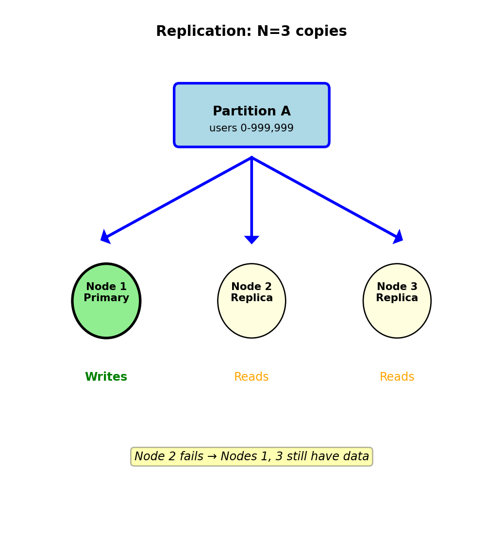
3 replicas = survive 2 simultaneous failures

Replication Creates Consistency Problem

Write must propagate from primary to replicas

Write flow:

Client sends write to Primary (Node 1)
Primary updates local copy
Primary sends update to Replicas (Nodes 2, 3)
Replicas acknowledge receipt

Network latencies:

Same datacenter: 1-5ms between nodes
Cross-datacenter: 50-200ms
Replica may be temporarily offline

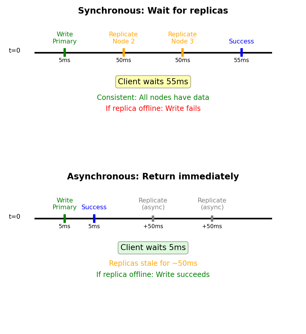
Critical question: When does write “succeed”?

Option A: Wait for all replicas (synchronous)

Client → Primary (5ms) → Wait for replicas (50ms)
Total latency: 55ms
If replica offline: Write fails
Result: All nodes have same data (consistent)

Option B: Return immediately (asynchronous)

Client → Primary (5ms) → Return success
Replicas updated in background (async)
Total latency: 5ms
If replica offline: Write still succeeds
Result: Replicas temporarily stale (inconsistent)

Trade-off: 5ms vs 55ms response time

Consistency vs latency vs availability trade-off

Network Partitions Split Clusters

Network partition = nodes cannot communicate due to network failure

Common causes:

Switch failure in datacenter
Fiber cable cut (construction accident)
Network misconfiguration
AWS documented frequency: ~0.1% of requests see partition effects

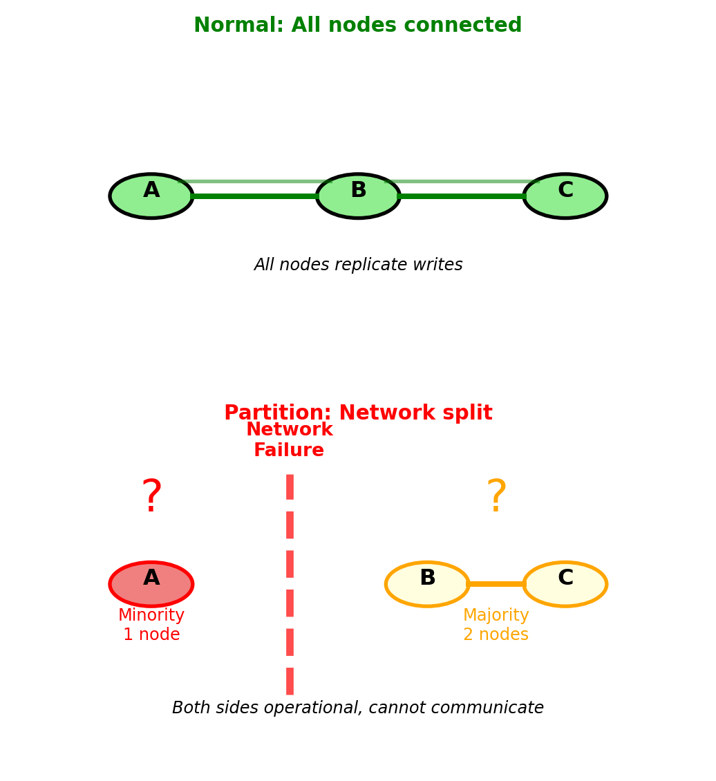
Example: 3-node cluster [A, B, C]

Normal operation:

All nodes communicate
Writes propagate A → B → C

Network partition occurs:

Network splits: [Node A] isolated from [Nodes B, C]
Both sides still operational
Both sides think they’re correct

Critical problem: Neither side knows if other side crashed or network failed

Duration:

Seconds: Brief network glitch
Minutes: Switch reboot
Hours: Waiting for human intervention (fiber repair)

During partition:

Both sides may accept writes
Creates conflicting data versions
Must resolve after partition heals

Partition forces choice: reject writes or accept conflicts

CAP Theorem Forces a Choice During Partitions

Three properties distributed systems want:

Consistency (C):

All nodes return same value for same query
Read always returns most recent write
No stale data

Availability (A):

Every request gets non-error response
No timeouts or failures
System always operational

Partition tolerance (P):

System works despite network splits
Required for any distributed system
Network failures inevitable

CAP Theorem: Cannot have all three during network partition

During partition, must choose:

CP (Consistency + Partition tolerance):

Reject requests to minority partition
Guarantees consistency
Sacrifices availability

AP (Availability + Partition tolerance):

Accept requests on all partitions
Guarantees availability
Sacrifices immediate consistency

Real systems:

Banking: CP (consistency critical)
Social media: AP (availability critical)
Inventory: CP (avoid overselling)
Analytics: AP (stale data acceptable)

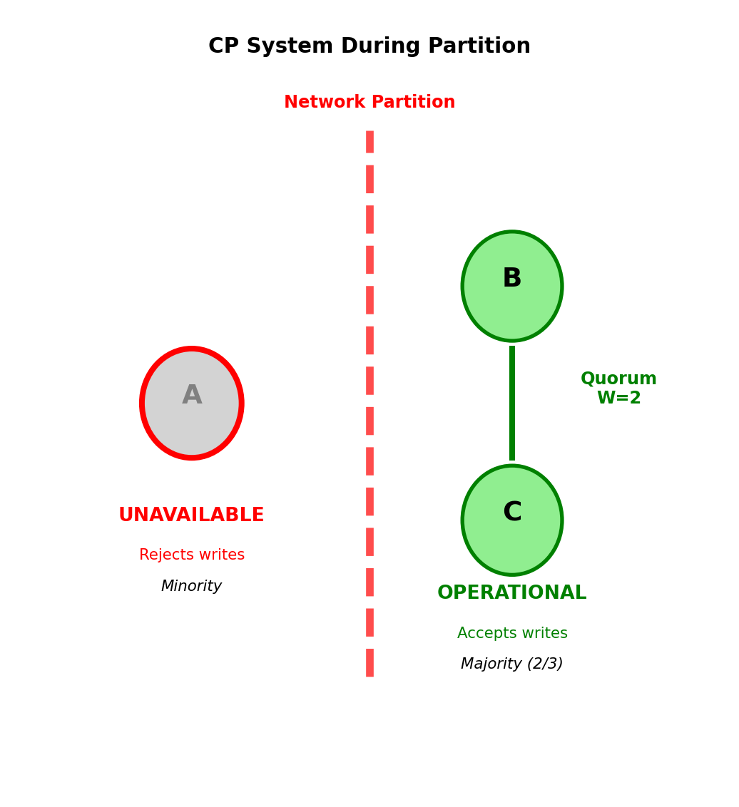
CP Systems Sacrifice Availability for Consistency

CP behavior during partition: [Node A] | [Nodes B, C]

Minority partition (Node A):

Rejects all write requests: “Error: Cannot reach majority”
May reject reads (depending on configuration)
Becomes unavailable to clients

Majority partition (Nodes B, C):

Continues accepting writes
Requires majority (2 of 3 nodes) for writes
Guarantees no conflicting data

After partition heals:

Node A syncs from B or C
No conflicts to resolve
Data guaranteed consistent

Write quorum: W > N/2

3 nodes: Must write to 2 nodes
Latency: Wait for slowest of 2 nodes
Cost: Higher latency, possible unavailability

PostgreSQL example:

Primary fails → replica promoted
Failover time: 30-120 seconds
During failover: All writes fail
After: Guaranteed consistency

Use CP when:

Financial transactions (no double-spending)
Inventory (no overselling)
User authentication (no conflicting state)

Trade-off: Latency and availability for guaranteed consistency

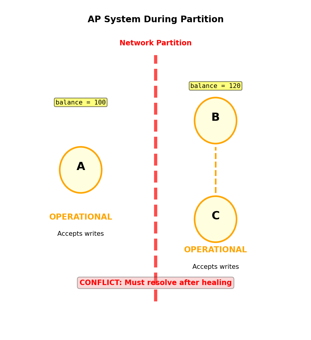
AP Systems Sacrifice Consistency for Availability

AP behavior during partition: [Node A] | [Nodes B, C]

Both partitions accept writes:

Node A: Accepts writes from its clients
Nodes B, C: Accept writes from their clients
Result: Divergent data versions

Example conflict:

Node A: user.balance = 100 (withdraw $50)
Node B: user.balance = 120 (deposit $20)
Initial: user.balance = 150

After partition heals: Which is correct?

Conflict resolution strategies:

1. Last-write-wins (timestamp):

Keep write with latest timestamp
Simple, fast
Risk: Clock skew causes wrong choice, data loss

2. Application merge:

Application logic combines conflicts
Example: Both transactions valid → balance = 70
Correct but complex

3. Vector clocks:

Track causality between writes
Detect concurrent writes
DynamoDB approach

Cassandra example:

Write with W=1 (any node): 5ms latency
Always available during partitions
Read may return stale data
Eventual consistency: Replicas converge in milliseconds to seconds

Trade-off: Consistency for availability and low latency

BASE Properties Define AP System Guarantees

ACID (relational databases):

Atomic: All or nothing
Consistent: Constraints enforced
Isolated: Concurrent transactions don’t interfere
Durable: Committed data survives failures

BASE (distributed systems):

Basically Available: System responds even during failures
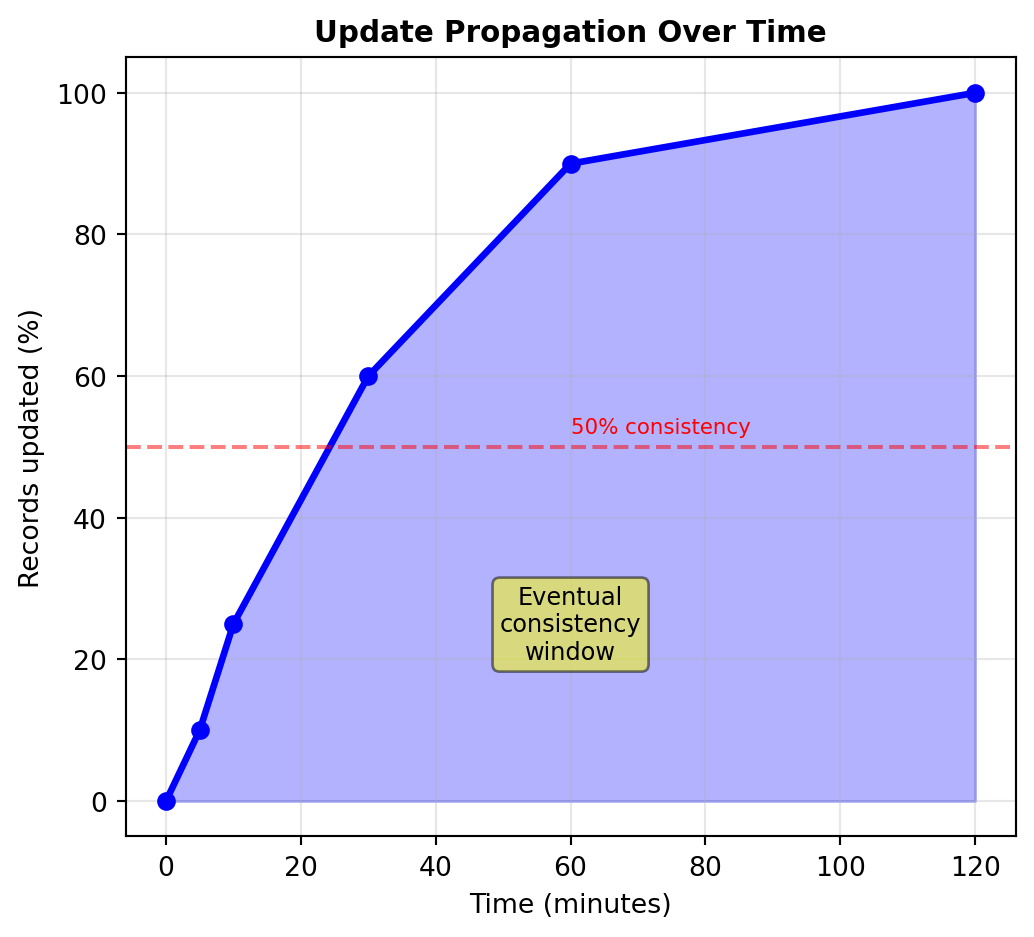
Soft state: State may change without input (due to eventual consistency)
Eventual consistency: Replicas converge given enough time

Basically Available:

System operational during network partitions
May return stale data or degraded service
Prioritizes availability over correctness

Soft State:

No guaranteed consistency at any given moment
State changes as updates propagate
Application must handle inconsistencies

Eventual Consistency:

All replicas converge to same value
Time window: milliseconds to seconds
No guarantee when convergence occurs

Practical implications:

Read from replica: May get old value
Write to one node: Other nodes lag behind
Network partition: Nodes diverge temporarily
Partition heals: Conflict resolution required

BASE trades immediate consistency for availability and partition tolerance (AP in CAP)

Tunable Consistency Balances Trade-offs

Modern systems allow per-query consistency level

Cassandra consistency levels:

ONE: Return after 1 replica responds

Latency: 5ms
Consistency: Eventual (may read stale)
Availability: High (works with 1 node)

QUORUM: Return after majority responds (R+W > N)

Latency: 20ms
Consistency: Strong (if W=QUORUM also)
Availability: Medium (needs majority alive)

ALL: Return after all replicas respond

Latency: 50ms
Consistency: Strong
Availability: Low (all nodes must be up)

DynamoDB read options:

Eventually consistent: 5ms, may be stale
Strongly consistent: 10ms, sees all writes

Application chooses per-query:

# Fast read for displaying comments (stale OK)
comments = db.query(
    consistency='ONE'  # 5ms, eventual
)

# Strong read for payment verification
balance = db.query(
    consistency='QUORUM'  # 20ms, consistent
)

Consistency vs latency trade-off:

Level	Replicas	Latency	Consistency	Availability
ONE	1	5ms	Eventual	High
QUORUM	2/3	20ms	Strong*	Medium
ALL	3/3	50ms	Strong	Low

*If write also uses QUORUM: R+W > N guarantees overlap

Quorum mathematics:

N = 3 replicas
W = 2 (write quorum)
R = 2 (read quorum)
R + W = 4 > N = 3
Guarantees: Read overlaps with write nodes

Latency distribution (Cassandra, same datacenter):

ONE: p50=5ms, p99=10ms
QUORUM: p50=20ms, p99=50ms
ALL: p50=50ms, p99=200ms

Application decides trade-off:

Social feed: ONE (fast, stale OK)
Shopping cart: QUORUM (consistent)
Account balance: ALL (critical accuracy)

Different consistency levels optimize different use cases within same system

Key-Value Stores

Key-Value Model - Dictionary at Database Scale

Fundamental abstraction:

PUT(key, value)  # Store
value = GET(key) # Retrieve
DELETE(key)      # Remove

Value is opaque blob:

Database does not interpret contents
No schema enforcement
No query language for value structure
Application handles serialization

Examples: Redis, Memcached, Riak, DynamoDB (key-value mode)

Why minimal structure:

O(1) lookup with hash function
Trivial horizontal partitioning
Minimal feature set reduces overhead
No query parser or optimizer

Contrast with relational:

Relational: Schema, types, constraints, indexes, query optimizer
Key-value: Hash table, bytes in/bytes out
Trade query capability for raw performance

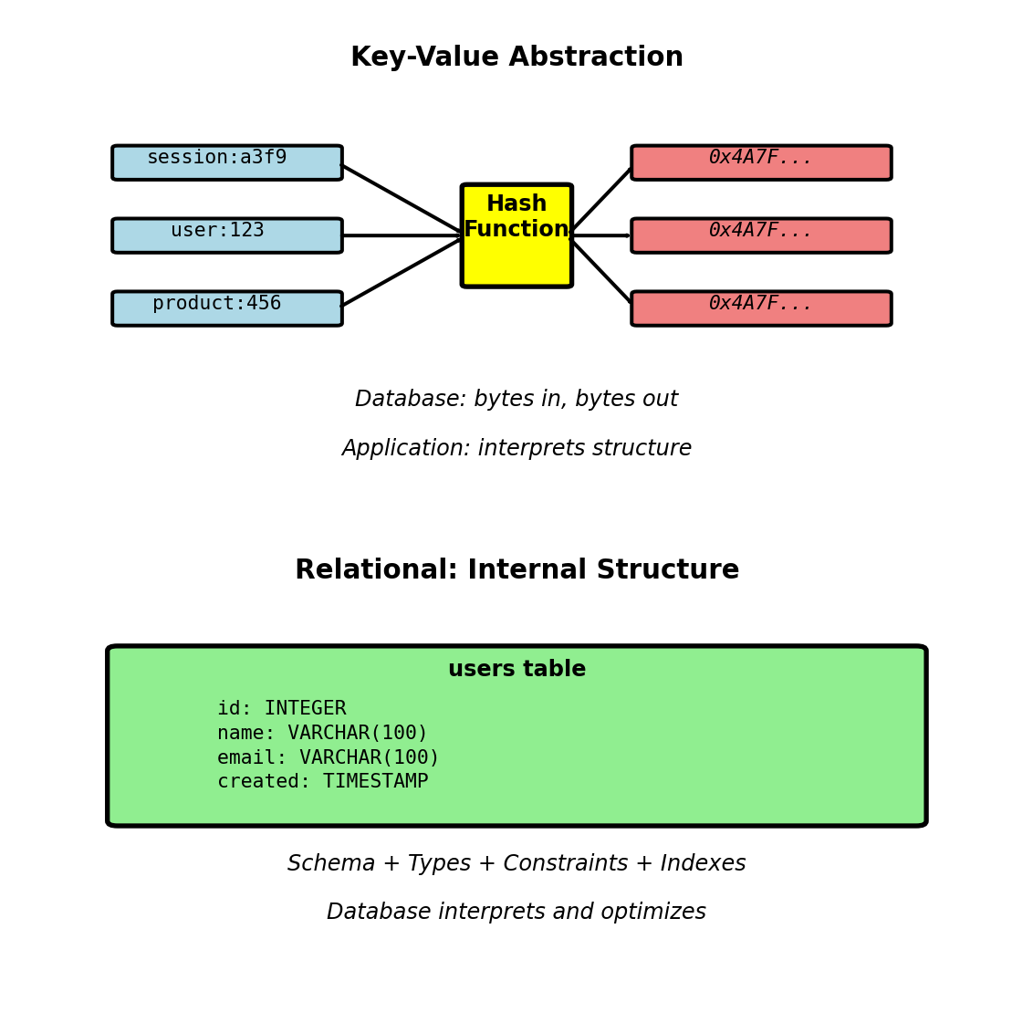
Simple interface provides O(1) access with minimal overhead

Operations Beyond GET/PUT

Core operations:

# Basic
redis.set("key", "value")
redis.get("key")
redis.delete("key")

# Conditional update
redis.setnx("key", "value")  # SET if Not eXists
redis.set("key", "new", xx=True)  # SET if exists

# Atomic counter
redis.incr("counter")  # Atomic increment
redis.decr("counter")  # Atomic decrement

# Time to live
redis.setex("session:abc", 1800, data)  # 30 min TTL
redis.expire("key", 3600)  # Set TTL on existing key

Advanced (Redis):

# Sorted sets for ranking
redis.zadd("leaderboard", {"player1": 1000})
rank = redis.zrank("leaderboard", "player1")

# Range queries on sorted keys
keys = redis.keys("session:*")  # Blocks server during scan
cursor, keys = redis.scan(0, match="session:*")  # Non-blocking iteration

Cannot do:

Query on value contents without retrieving
Secondary indexes
Joins across keys
Aggregations without application logic

Example session showing operations:

#| echo: true
#| eval: false

# Store session with 30-minute expiration
import redis
import json

r = redis.Redis()

session_data = {
    "user_id": 123,
    "login_time": "2025-01-15T10:30:00Z",
    "cart": ["product_456", "product_789"]
}

# Store
r.setex(
    "session:a3f9b2c1",
    1800,  # 30 minutes
    json.dumps(session_data)
)

# Retrieve
data = r.get("session:a3f9b2c1")
if data:
    session = json.loads(data)
    print(f"User {session['user_id']} logged in")
else:
    print("Session expired or not found")

# Extend TTL
r.expire("session:a3f9b2c1", 1800)

# After 30 minutes: automatic deletion
# No polling, no cleanup jobs required

Operations execute in microseconds

Must know exact key for retrieval

Session Management with Automatic Expiration

Web application session requirements:

Store per-user state (user_id, preferences, cart)
Expire after inactivity (30 minutes typical)
High volume (every HTTP request checks session)
Fast access (< 5ms latency requirement)

Relational approach problems:

CREATE TABLE sessions (
  session_id VARCHAR(64) PRIMARY KEY,
  user_id INT,
  data JSONB,
  created_at TIMESTAMP,
  last_activity TIMESTAMP
);

-- Every request
SELECT * FROM sessions
WHERE session_id = ?
  AND last_activity > NOW() - INTERVAL '30 minutes';

-- Cleanup job (runs every minute)
DELETE FROM sessions
WHERE last_activity < NOW() - INTERVAL '30 minutes';

Issues:

Cleanup job scans millions of rows
Index on last_activity, but still expensive
Delete locks table
Write amplification: Record activity on every request

Key-value with TTL:

# Store with automatic expiration
redis.setex(f"session:{token}", 1800, session_data)

# Retrieve (no expiration check needed)
data = redis.get(f"session:{token}")

# Extend session on activity
if data:
    redis.expire(f"session:{token}", 1800)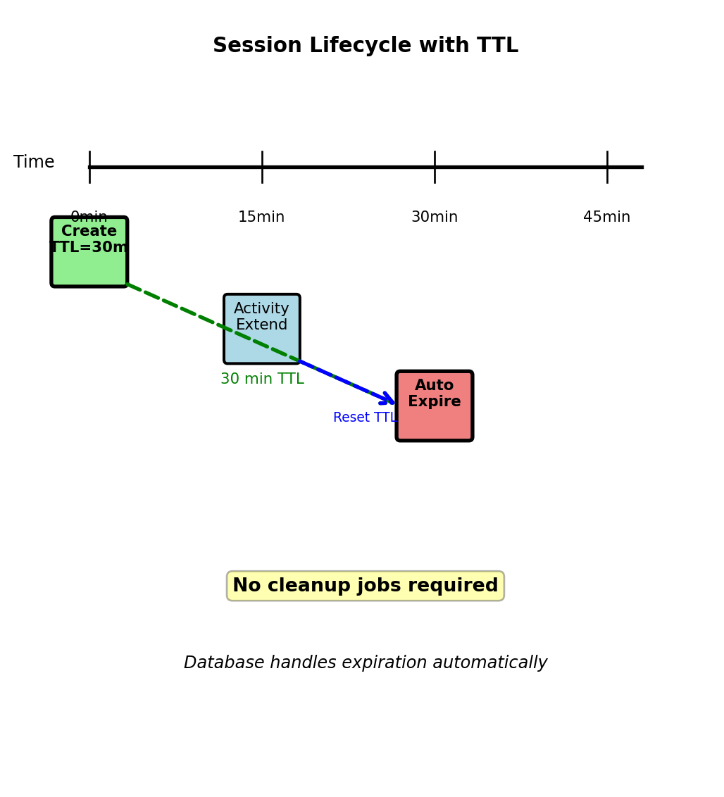

Performance:

Session check: < 1ms (in-memory)
Relational: 10-50ms (disk, index lookup, expiration check)
Automatic cleanup vs periodic scan

Value Serialization - Application Choice

Database stores bytes, application chooses format:

JSON - Human readable:

session = {
    "user_id": 123,
    "cart": ["product_456", "product_789"],
    "preferences": {"theme": "dark"},
    "login_time": "2025-01-15T10:30:00Z"
}
value = json.dumps(session)
# Size: 147 bytes
# Parse time: ~50 microseconds

MessagePack - Binary efficient:

import msgpack
value = msgpack.packb(session)
# Size: 89 bytes (39% smaller)
# Parse time: ~20 microseconds

Protocol Buffers - Typed schema:

message Session {
  int32 user_id = 1;
  repeated string cart = 2;
  map<string, string> preferences = 3;
  string login_time = 4;
}

value = session_pb.SerializeToString()
# Size: 68 bytes (54% smaller)
# Parse time: ~15 microseconds
# Schema evolution support

Trade-offs:

JSON:

Debug with redis-cli
Language interop trivial
Larger size
Slower parse

MessagePack:

Opaque in redis-cli
Smaller, faster
Language support good
No schema definition

Protocol Buffers:

Smallest, fastest
Schema migration paths
Requires .proto files
Build step required

Most applications: JSON for simplicity

High-throughput systems: Binary formats

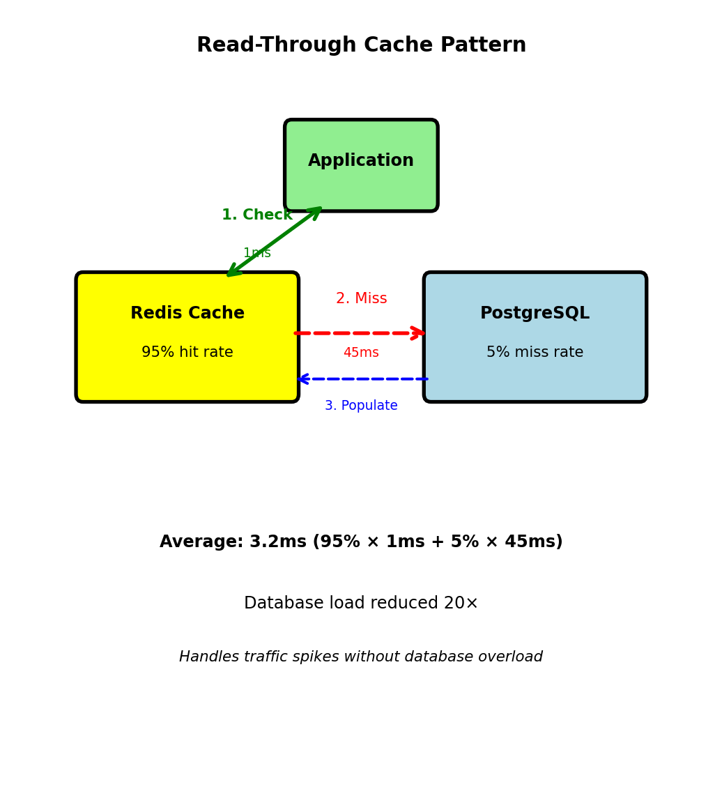
Caching Database Queries - Read-Through Pattern

Product catalog query:

SELECT p.*, c.name AS category_name
FROM products p
  JOIN categories c ON p.category_id = c.category_id
WHERE p.product_id = 456;

Execution time: 45ms (JOIN, disk I/O)

Cache layer intercepts:

def get_product(product_id):
    cache_key = f"product:{product_id}"

    # Check cache
    cached = redis.get(cache_key)
    if cached:
        return json.loads(cached)  # 1ms

    # Cache miss - query database
    product = db.execute("""
        SELECT p.*, c.name AS category_name
        FROM products p
        JOIN categories c ON p.category_id = c.category_id
        WHERE p.product_id = ?
    """, product_id)  # 45ms

    # Cache result for 5 minutes
    redis.setex(cache_key, 300, json.dumps(product))

    return product

Performance calculation:

Cache hit rate: 95%
Average latency: 0.95 × 1ms + 0.05 × 45ms = 3.2ms
vs without cache: 45ms
14× faster average response

Database load reduction:

1000 requests/second
Without cache: 1000 database queries/second
With 95% hit rate: 50 database queries/second
20× reduction in database load

Cache absorbs read load

Database handles writes and cache misses

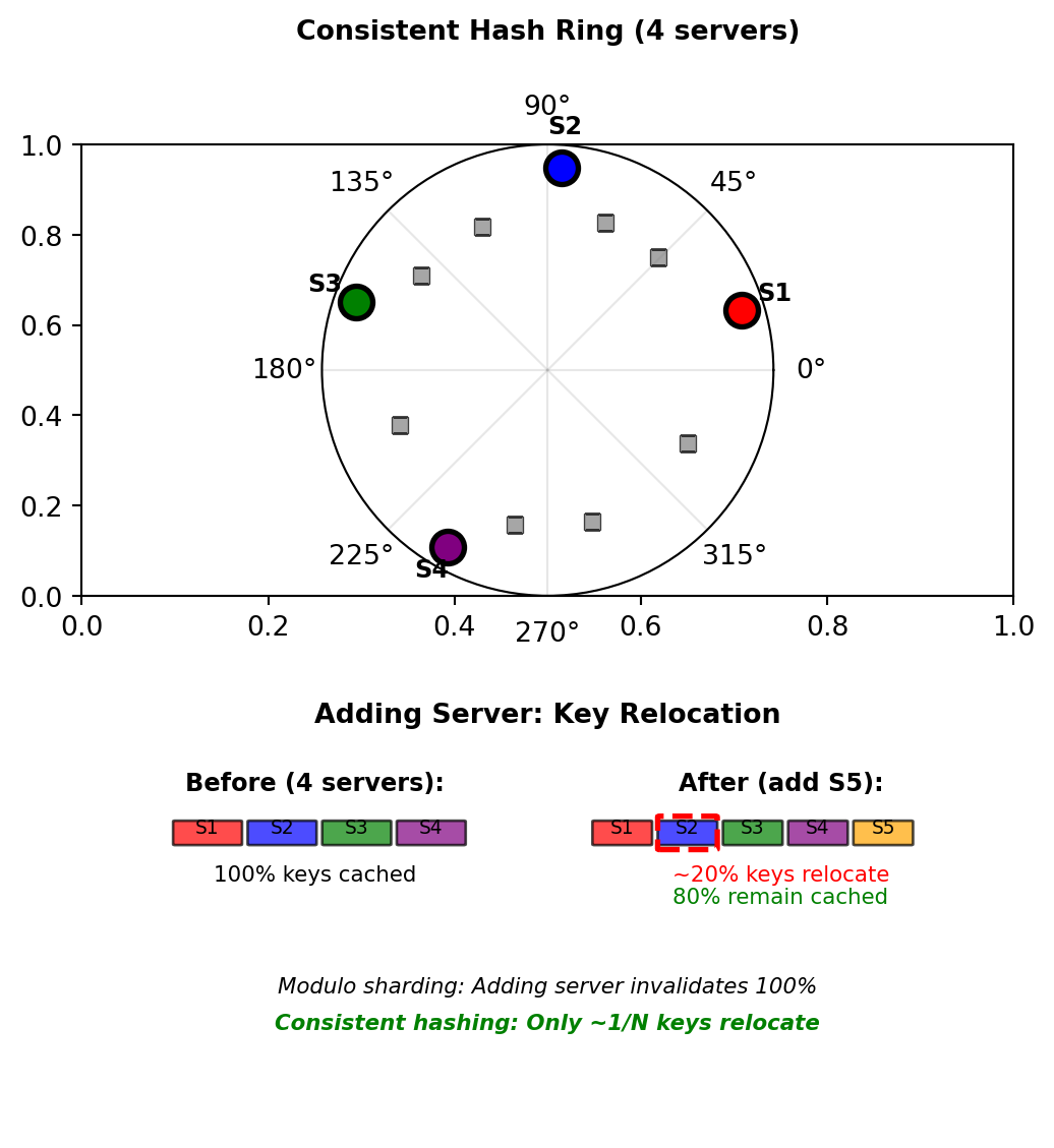
Distributed Caching with Consistent Hashing

Single cache server limit:

64GB RAM = ~50M cached items
Network bandwidth: 10Gbps
Need horizontal scaling

Naive sharding breaks:

server_id = hash(key) % N  # N = number of servers

Adding server changes N → all keys remap

Consistent hashing solution:

Hash ring: 0 to 2³²-1
Servers and keys both hash to ring positions
Key stored on next clockwise server
Adding server: Only adjacent keys relocate (~1/N)

Example with 4 servers:

# Server positions on ring (hash of server ID)
servers = {
    "server1": hash("server1") % (2**32),  # 428312345
    "server2": hash("server2") % (2**32),  # 1827364829
    "server3": hash("server3") % (2**32),  # 2913746582
    "server4": hash("server4") % (2**32),  # 3728191028
}

# Key placement
key_hash = hash("product:456") % (2**32)  # 945628371
# Finds next server clockwise: server2

Adding server5:

New position: 2100000000
Only keys between server2 and server5 relocate
~25% of keys move (1/4 servers)
Other 75% remain cached

Hash slots distribute cache load without global invalidation

Rate Limiting with Atomic Counters

API rate limit: 100 requests per minute per user

Wrong approach - Race condition:

# Read current count
count = int(redis.get(f"rate:{user_id}") or 0)

# Check limit
if count >= 100:
    return "Rate limit exceeded"

# Increment count
redis.set(f"rate:{user_id}", count + 1)
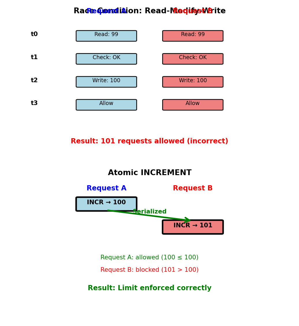
redis.expire(f"rate:{user_id}", 60)

Problem with concurrent requests:

Time    Request A           Request B
t0      Read count=99       Read count=99
t1      Check: 99 < 100     Check: 99 < 100
t2      Set count=100       Set count=100
t3      Allow request       Allow request

Both requests see count=99, both allowed → 101 requests

Correct approach - Atomic operation:

key = f"rate:{user_id}:{current_minute}"

# Atomic increment returns new value
count = redis.incr(key)

# Set TTL on first request
if count == 1:
    redis.expire(key, 60)

# Check after increment
if count > 100:
    return "Rate limit exceeded"

return "Request allowed"

Atomic increment guarantees correct count under concurrency

Single round-trip, no race conditions

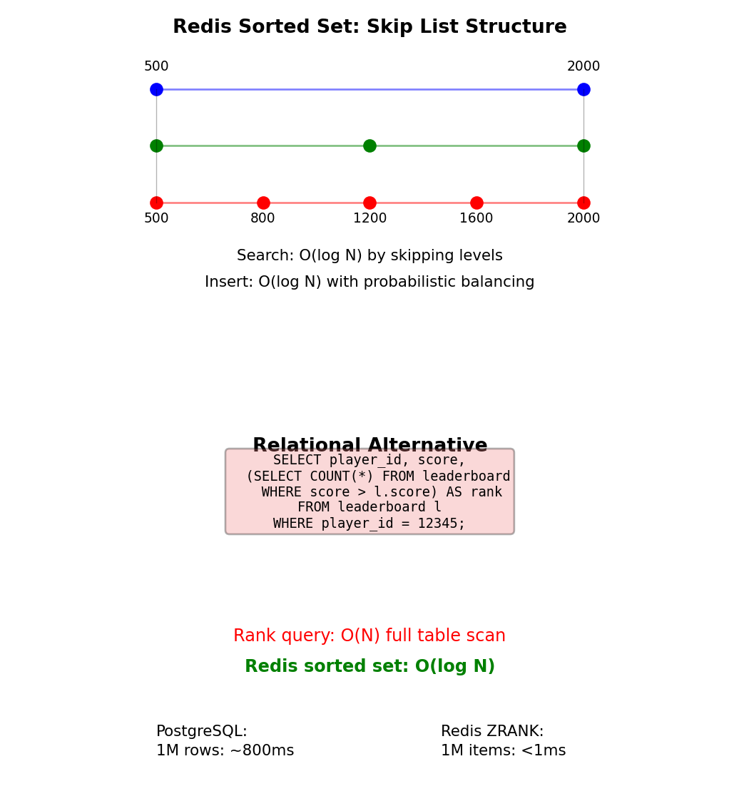
Leaderboards with Sorted Sets

Gaming leaderboard requirements:

Rank 1 million players by score
Update scores frequently (every game completion)
Query operations:
- Player rank: “What rank is player_id=12345?”
- Top N: “Who are top 10 players?”
- Score range: “Players with 1000-2000 points”

Redis sorted set:

import redis
r = redis.Redis()

# Update player score (O(log N))
r.zadd("leaderboard", {"player_12345": 1850})
r.zadd("leaderboard", {"player_67890": 2100})

# Get player rank - 0-indexed, from lowest (O(log N))
rank = r.zrevrank("leaderboard", "player_12345")
# Returns: 43127 (meaning 43,128th place)

# Get top 10 players with scores (O(log N + 10))
top_10 = r.zrevrange("leaderboard", 0, 9, withscores=True)
# Returns: [("player_67890", 2100.0), ...]

# Get players in score range (O(log N + M))
players = r.zrangebyscore("leaderboard", 1000, 2000)

# Get player score (O(1))
score = r.zscore("leaderboard", "player_12345")

All operations logarithmic or better with 1M players

Internal structure: Skip list

Specialized data structure for ranking operations

Key-Value Limitations

Cannot query on value contents:

All sessions for user:

# Need to track session keys separately
redis.sadd(f"user_sessions:{user_id}", session_id)

# Or scan all keys (expensive)
cursor = 0
sessions = []
while True:
    cursor, keys = redis.scan(cursor, match="session:*")
    for key in keys:
        data = json.loads(redis.get(key))
        if data["user_id"] == target_user:
            sessions.append(data)
    if cursor == 0:
        break
# Scans entire keyspace, O(N) operation

Products under $20:

# Impossible without secondary index
# Must maintain separate sorted set
redis.zadd("products_by_price", {product_id: price})
cheap = redis.zrangebyscore("products_by_price", 0, 20)

Application must manually maintain indexes

No relationships:

# Get user and their orders - two queries
user = json.loads(redis.get(f"user:{user_id}"))
order_ids = json.loads(redis.get(f"user_orders:{user_id}"))
orders = [json.loads(redis.get(f"order:{oid}")) for oid in order_ids]

No JOIN operation

No multi-key transactions (usually):

Redis transactions limited:

# WATCH/MULTI/EXEC for optimistic locking
redis.watch("account:A", "account:B")
balance_a = redis.get("account:A")
balance_b = redis.get("account:B")

pipe = redis.pipeline()
pipe.set("account:A", balance_a - 100)
pipe.set("account:B", balance_b + 100)
result = pipe.execute()  # Fails if watched keys modified

DynamoDB: 25 item transaction limit

When key-value is wrong:

Complex queries on attributes
Relationships between entities
Consistency across multiple items
Need secondary indexes on value fields

When key-value is right:

Known exact key for access
Simple GET/PUT operations dominate
High throughput, low latency required
Data can be denormalized per key
Temporary or cached data

Key-value complements relational, does not replace

Document Databases

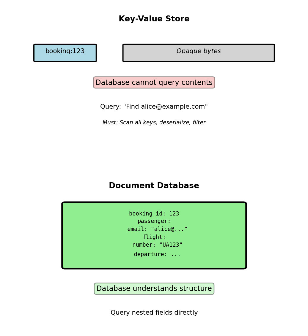
Document Model - Structured Objects as Storage Unit

Document database stores structured objects as atomic units

Recall embed vs reference patterns from earlier. Document databases implement these patterns while understanding document structure.

Key-value limitation:

# Key-value: Opaque blob
redis.set("booking:123", json.dumps(booking_data))
value = redis.get("booking:123")
booking = json.loads(value)  # Application interprets

# Cannot query: "Find bookings for alice@example.com"
# Must scan all keys and deserialize

Document database capability:

// Database understands structure
db.bookings.find({
  "passenger.email": "alice@example.com"
})
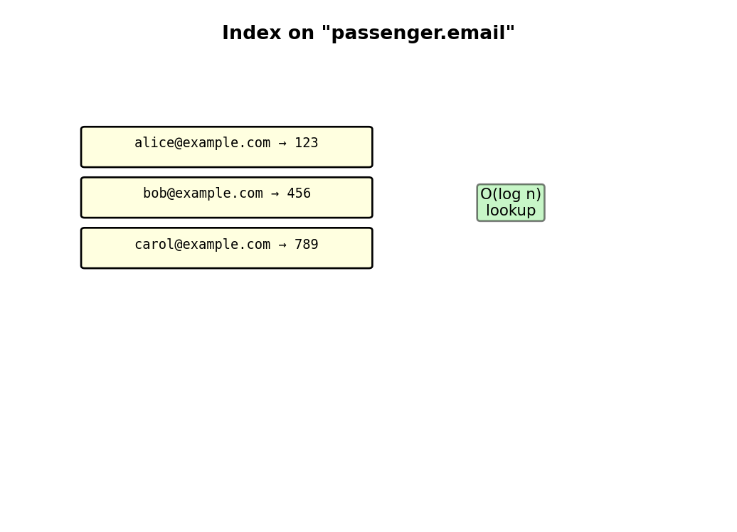
// Direct query on nested field

Database parses JSON structure to support:

Queries on nested fields without deserialization
Indexes on any field, including nested
Aggregations across document contents
Structure validation

Primary implementations: MongoDB (BSON), CouchDB (JSON), DocumentDB

Document databases bridge gap between key-value flexibility and relational query power

MongoDB Collections and Documents

Collection: Group of related documents (analogous to relational table)

Document: Single JSON object with _id primary key

No enforced schema: Documents in same collection can have different fields

Booking collection example:

{
  "_id": ObjectId("507f1f77bcf86cd799439011"),
  "booking_reference": "ABC123",
  "passenger_id": 123,
  "flight_id": 456,
  "seat": "12A",
  "booking_time": ISODate("2025-01-15T10:30:00Z"),
  "price": 450.00
}

MongoDB-specific types:

ObjectId: 12-byte unique identifier (timestamp + random)
ISODate: Native datetime type (UTC)
NumberLong, NumberDecimal: Typed numeric values
Embedded documents and arrays

Storage format: BSON (Binary JSON)

Binary encoding: More efficient than text JSON
Additional types: Date, Binary, Decimal128, ObjectId
Preserves field order (unlike JSON spec)
~1.5× space overhead vs raw JSON for typical documents

Collection contains documents with varying fields

Querying Nested Fields - Dot Notation

Relational limitation: Accessing nested data required JOINs

Document structure with nesting:

{
  "booking_id": 12345,
  "passenger": {
    "name": "Alice Chen",
    "email": "alice@example.com",
    "frequent_flyer": {
      "number": "FF123456",
      "tier": "Gold",
      "miles": 85000
    }
  },
  "flight": {
    "number": "UA123",
    "departure_airport": "LAX",
    "scheduled_departure": ISODate("2025-02-15T14:30:00Z")
  }
}

Dot notation queries:

// Find bookings for specific email
db.bookings.find({
  "passenger.email": "alice@example.com"
})

// Query nested 3 levels deep
db.bookings.find({
  "passenger.frequent_flyer.tier": "Gold"
})

// Combine nested and top-level filters
db.bookings.find({
  "flight.departure_airport": "LAX",
  "flight.scheduled_departure": {
    $gte: ISODate("2025-02-01"),
    $lt: ISODate("2025-03-01")
  }
})

Index on nested field:

db.bookings.createIndex({"passenger.email": 1})

Query execution with index:

Nested field indexed like top-level field
B-tree lookup: O(log n)
1M documents: ~2ms query time

Comparison to relational approach:

-- Requires 2 JOINs for same data
SELECT b.*
FROM bookings b
  JOIN passengers p ON b.passenger_id = p.passenger_id
  JOIN frequent_flyer ff ON p.passenger_id = ff.passenger_id
WHERE p.email = 'alice@example.com'
  AND ff.tier = 'Gold';

Performance measurement (1M bookings):

Document nested query: 2ms
Relational 2-JOIN query: 15ms
Difference: JOIN operation cost (hash join on 1M rows)

Why faster:

Document: Single index lookup + fetch
Relational: Index lookup + JOIN build + JOIN probe

Nested data stored contiguously eliminates JOIN cost

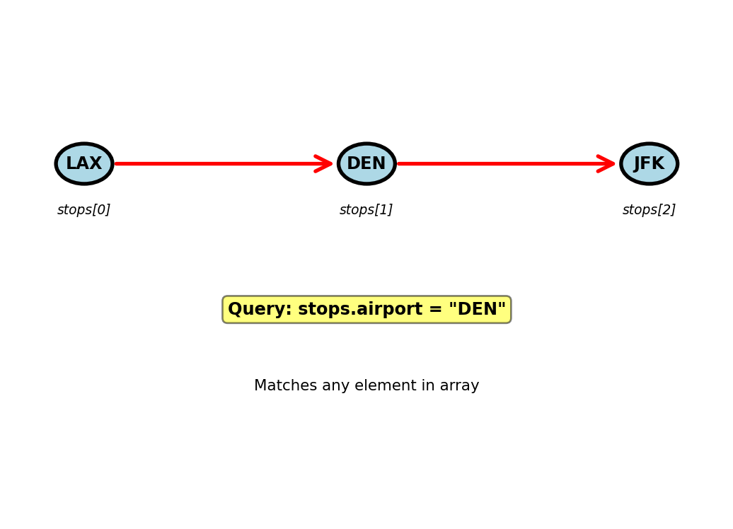
Querying Arrays - Flight Stops Example

Scenario: Multi-stop flights (LAX → DEN → JFK)

{
  "flight_id": 789,
  "flight_number": "UA456",
  "stops": [
    {
      "airport": "LAX",
      "arrival": null,
      "departure": ISODate("2025-02-15T08:00:00Z"),
      "gate": "B12"
    },
    {
      "airport": "DEN",
      "arrival": ISODate("2025-02-15T10:30:00Z"),
      "departure": ISODate("2025-02-15T11:00:00Z"),
      "gate": "A5"
    },
    {
      "airport": "JFK",
      "arrival": ISODate("2025-02-15T17:00:00Z"),
      "departure": null,
      "gate": "C8"
    }
  ]
}

Query any array element:

// Find all flights stopping at DEN
db.flights.find({
  "stops.airport": "DEN"
})
// Matches if ANY element has airport: "DEN"

Query specific array position:

// First stop must be LAX
db.flights.find({
  "stops.0.airport": "LAX"
})

Match array element with multiple conditions:

// Find flights with DEN stop, departure after 11:00
db.flights.find({
  "stops": {
    $elemMatch: {
      "airport": "DEN",
      "departure": {$gte: ISODate("2025-02-15T11:00:00Z")}
    }
  }
})

Array operators:

$elemMatch: Element meets multiple conditions
$all: Array contains all specified elements
$size: Array has specific length
$: Positional operator for updates

Array queries operate across all elements

Indexes on Nested Fields and Arrays

Creating indexes on document structure:

// Index on nested field (2 levels deep)
db.bookings.createIndex({"passenger.email": 1})

// Compound index across nesting levels
db.bookings.createIndex({
  "flight.departure_airport": 1,
  "flight.scheduled_departure": 1
})

Multikey indexes on arrays:

// Index on array field
db.flights.createIndex({"stops.airport": 1})

// Flight with 3 stops creates 3 index entries:
// "LAX" → flight_id: 789
// "DEN" → flight_id: 789
// "JFK" → flight_id: 789

Query execution:

// With index (fast)
db.bookings.find({"passenger.email": "alice@example.com"})
// Index seek: O(log n), ~2ms for 1M documents

// Without index (slow)
db.bookings.find({"passenger.phone": "+1-555-0123"})
// Collection scan: O(n), ~500ms for 1M documents

Index size impact:

Nested field indexes: Same cost as top-level
Multikey (array) indexes: Size = sum of array lengths across collection
10K flights × 3 stops average = 30K index entries

MongoDB limit: 64 indexes per collection

Indexes work on any document field

Performance (1M documents): Indexed query: 2ms, Collection scan: 500ms

Aggregation Pipeline - Multi-Stage Processing

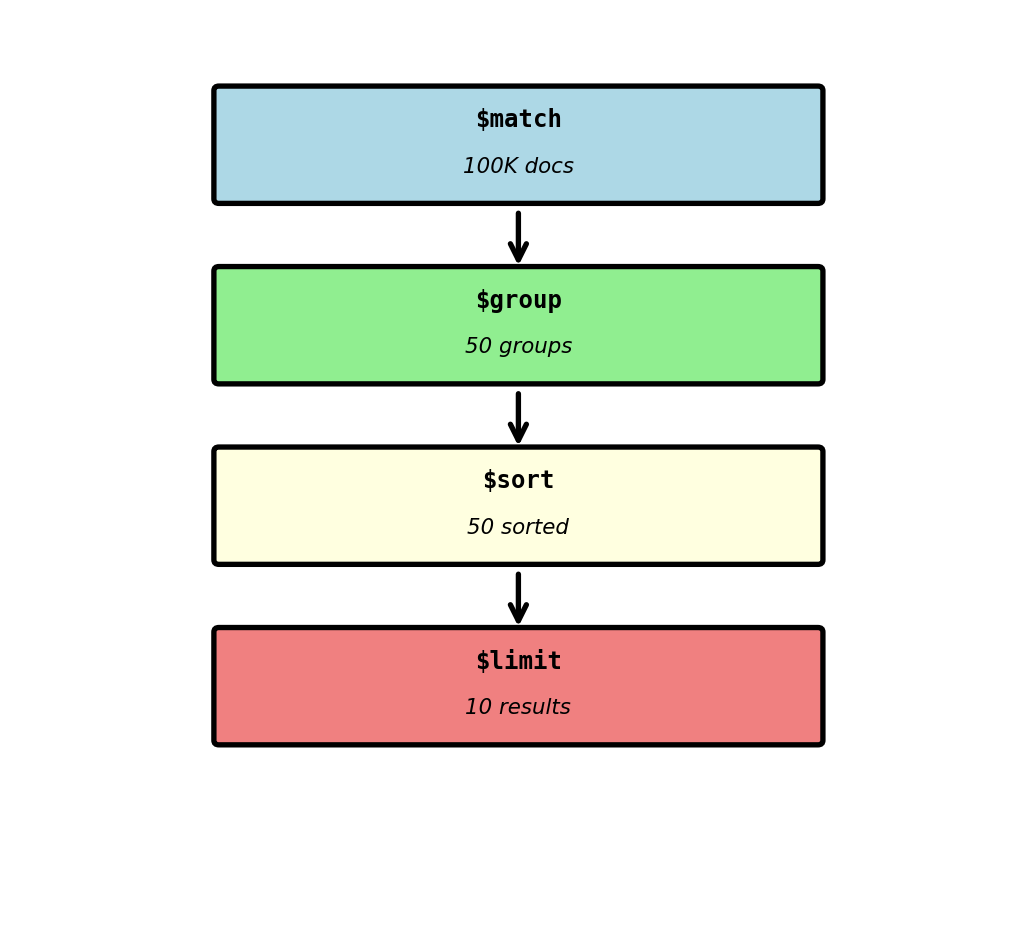
Query: “Average booking price by departure airport for last 30 days”

Relational approach requires JOIN:

SELECT f.departure_airport, AVG(b.price)
FROM bookings b
JOIN flights f ON b.flight_id = f.flight_id
WHERE b.booking_time >= CURRENT_DATE - INTERVAL '30 days'
GROUP BY f.departure_airport
ORDER BY AVG(b.price) DESC
LIMIT 10;

MongoDB aggregation pipeline:

db.bookings.aggregate([
  // Stage 1: Filter to last 30 days
  {
    $match: {
      booking_time: {
        $gte: ISODate("2025-01-15"),
        $lt: ISODate("2025-02-15")
      }
    }
  },

  // Stage 2: Group by departure airport
  {
    $group: {
      _id: "$flight.departure_airport",
      avg_price: {$avg: "$price"},
      total_bookings: {$sum: 1},
      min_price: {$min: "$price"},
      max_price: {$max: "$price"}
    }
  },

  // Stage 3: Sort by average price descending
  {
    $sort: {avg_price: -1}
  },

  // Stage 4: Limit to top 10
  {
    $limit: 10
  }
])

Result:

[
  {
    "_id": "LAX",
    "avg_price": 487.50,
    "total_bookings": 2500,
    "min_price": 250.00,
    "max_price": 950.00
  },
  {
    "_id": "JFK",
    "avg_price": 465.25,
    "total_bookings": 2100,
    "min_price": 275.00,
    "max_price": 875.00
  }
]

Pipeline processes documents through stages on database server

Aggregation - Unwind for Array Processing

Problem: Analyze which airports have most stops (connection hubs)

Document with stops array:

{
  "flight_number": "UA456",
  "departure": "LAX",
  "arrival": "JFK",
  "stops": ["LAX", "DEN", "JFK"]
}

Pipeline with $unwind:

db.flights.aggregate([
  // Stage 1: Expand stops array
  {
    $unwind: "$stops"
  },
  // After $unwind, creates 3 documents:
  // {flight_number: "UA456", stops: "LAX"}
  // {flight_number: "UA456", stops: "DEN"}
  // {flight_number: "UA456", stops: "JFK"}

  // Stage 2: Group by airport
  {
    $group: {
      _id: "$stops",
      flight_count: {$sum: 1}
    }
  },

  // Stage 3: Sort by frequency
  {
    $sort: {flight_count: -1}
  },

  // Stage 4: Top 10 airports
  {
    $limit: 10
  }
])

Result:

[
  {"_id": "DEN", "flight_count": 2500},
  {"_id": "ORD", "flight_count": 2100},
  {"_id": "ATL", "flight_count": 1900},
  {"_id": "DFW", "flight_count": 1750}
]

$unwind document explosion:

Array expansion multiplies document count:

Input: 10K flight documents
Average 3 stops per flight
After $unwind: 30K documents in pipeline
Memory: 30K × 1KB = 30MB buffered

Optimization: filter before unwind

db.flights.aggregate([
  {$match: {departure_date: {$gte: ISODate("2025-02-01")}}},  // Filter first
  {$unwind: "$stops"},
  {$group: {_id: "$stops", flight_count: {$sum: 1}}}
])

Pipeline size:

Filter reduces 10K → 2K flights
Unwind creates 2K × 3 = 6K documents
5× memory reduction vs unwind-first

Measured performance:

Unwind-first: 850ms, 30MB peak memory
Filter-first: 180ms, 6MB peak memory

$unwind before $match creates unnecessary work

Schema Validation - Optional Enforcement

Problem: No schema enforcement - errors undetected

Typo: emial instead of email
Wrong type: "123" instead of 123
Missing required field

MongoDB JSON Schema validation:

db.createCollection("bookings", {
  validator: {
    $jsonSchema: {
      bsonType: "object",
      required: ["booking_reference", "passenger_id",
                 "flight_id", "price"],
      properties: {
        booking_reference: {
          bsonType: "string",
          pattern: "^[A-Z]{3}[0-9]{3}$",
          description: "Format: ABC123"
        },
        passenger_id: {
          bsonType: "int",
          minimum: 1
        },
        price: {
          bsonType: "decimal",
          minimum: 0,
          maximum: 10000
        },
        passenger: {
          bsonType: "object",
          properties: {
            email: {
              bsonType: "string",
              pattern: "^.+@.+\\..+$"
            }
          }
        }
      }
    }
  },
  validationAction: "error"  // or "warn"
})

Validation behavior:

Valid insert succeeds:

db.bookings.insertOne({
  booking_reference: "ABC123",
  passenger_id: 123,
  flight_id: 456,
  price: NumberDecimal("450.00")
})
// Success

Invalid insert rejected:

db.bookings.insertOne({
  booking_reference: "INVALID",  // Wrong pattern
  passenger_id: "123",           // Wrong type
  price: -50.00                  // Below minimum
})
// Error: Document failed validation

Validation options:

validationAction: "error" - Reject invalid documents
validationAction: "warn" - Log warning, allow insert
validationLevel: "moderate" - Validate only new/updated documents

Trade-off:

Validation = Type safety, data quality
No validation = Maximum flexibility, faster writes
Can enable per-collection based on requirements

Validation provides safety without rigid schema

Update Operations - Document Granularity

Updating nested fields:

// Update single nested field
db.bookings.updateOne(
  {booking_id: 12345},
  {$set: {"passenger.email": "alice.new@example.com"}}
)
// Only passenger.email changes, rest untouched

Updating array elements:

// Update element by position
db.flights.updateOne(
  {flight_id: 789},
  {$set: {"stops.1.departure": ISODate("2025-02-15T11:30:00Z")}}
)
// stops[1].departure updated

// Update element by condition ($ positional operator)
db.flights.updateOne(
  {flight_id: 789, "stops.airport": "DEN"},
  {$set: {"stops.$.departure": ISODate("2025-02-15T11:30:00Z")}}
)
// Updates first matching element

Update operators:

// Set field value
{$set: {field: value}}

// Remove field
{$unset: {field: ""}}

// Increment number
{$inc: {available_seats: -1}}

// Add to array
{$push: {tags: "premium"}}

// Remove from array
{$pull: {tags: "economy"}}

Atomicity guarantees:

Single document updates are atomic:

// Atomic: Decrement seats and add booking
db.flights.updateOne(
  {flight_id: 456, available_seats: {$gt: 0}},
  {
    $inc: {available_seats: -1},
    $push: {recent_bookings: booking_id}
  }
)
// Both operations succeed or both fail

Cross-document operations not atomic (without transactions):

// NOT atomic without transaction
db.flights.updateOne({flight_id: 456}, {$inc: {available_seats: -1}})
db.bookings.insertOne({flight_id: 456, ...})
// Second operation can fail, leaving inconsistent state

MongoDB 4.0+: Multi-document transactions

session = db.getMongo().startSession()
session.startTransaction()
try {
  session.getDatabase("airline").flights.updateOne(...)
  session.getDatabase("airline").bookings.insertOne(...)
  session.commitTransaction()
} catch (error) {
  session.abortTransaction()
}

Performance: Transactions add overhead (~2-3× slower)

Single-document atomicity sufficient for most embedded designs

Document Size Limits and Denormalization Trade-offs

MongoDB document constraints:

Maximum document size: 16MB
Maximum nesting depth: 100 levels
No hard limit on array length (constrained by 16MB total)

When embedding breaks:

Flight with all bookings embedded:

{
  "flight_id": 456,
  "flight_number": "UA123",
  "departure_airport": "LAX",
  "bookings": [
    {...},  // 1KB per booking
    {...},  // 200 bookings = 200KB
    {...}   // Still under 16MB
  ]
}

Problems at scale:

Works for 200 bookings (200KB < 16MB)
Each booking addition rewrites entire 200KB document
Concurrent booking updates conflict (document-level locking)
180-seat plane sold out: 180 document rewrites
Reading flight details loads unnecessary 200KB

When to reference instead of embed:

Unbounded growth (user’s order history over years)
Independent access patterns (query bookings without flight)
High update frequency (seat assignments change constantly)
Size exceeds reasonable threshold (>100KB per document)

Reference pattern (normalized approach):

// Flight document (small, stable)
{
  "flight_id": 456,
  "flight_number": "UA123",
  "departure_airport": "LAX",
  "arrival_airport": "JFK",
  "scheduled_departure": ISODate("2025-02-15T14:30:00Z"),
  "seats_available": 12,
  "total_seats": 180
}
// Size: 1KB

// Booking documents (separate collection)
{
  "booking_id": 789,
  "flight_id": 456,  // Reference
  "passenger_id": 123,
  "seat": "12A"
}
// 180 separate documents

Query patterns:

// Get flight: 1KB fetch
db.flights.findOne({flight_id: 456})

// Get bookings: Separate query
db.bookings.find({flight_id: 456})

// Add booking: Small update
db.bookings.insertOne({...})
db.flights.updateOne(
  {flight_id: 456},
  {$inc: {seats_available: -1}}
)

Reference when size or update patterns break embedding

MongoDB in Production - Replica Sets

Single server limitations:

Hardware failure → data loss
Maintenance → downtime
No geographic distribution
Read throughput limited to single machine

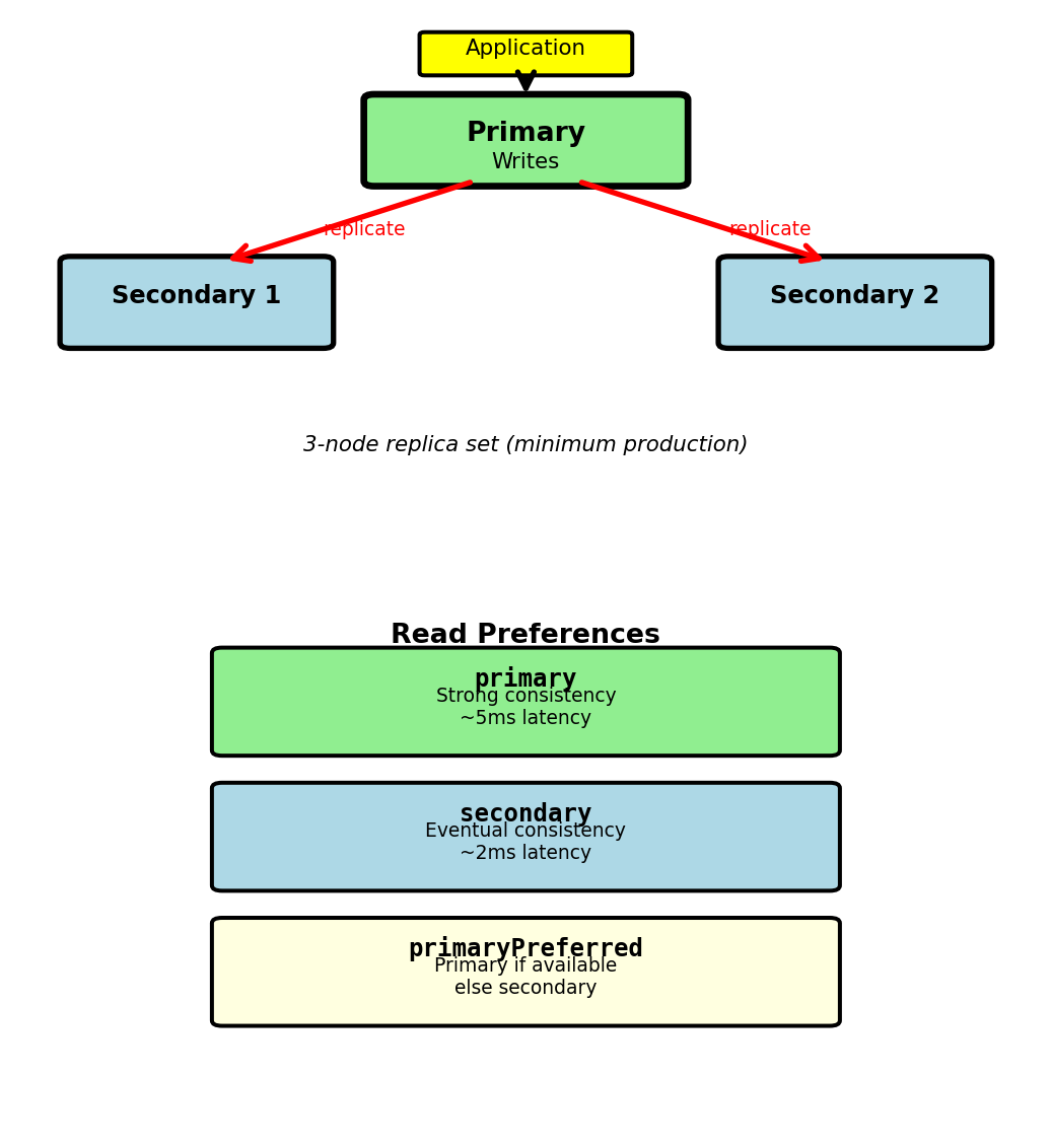
Replica set architecture:

Primary node: Handles all writes
Secondary nodes (2+): Replicate from primary
Automatic failover: Secondary elected if primary fails
Production minimum: 3 nodes (1 primary + 2 secondaries)

Write path:

// Application writes to primary
db.bookings.insertOne({...})

// Primary writes to oplog (operation log)
// Secondaries tail oplog and apply operations
// Replication asynchronous by default

Write concern controls durability:

// Wait for majority acknowledgment (2 of 3 nodes)
db.bookings.insertOne(
  {...},
  {writeConcern: {w: "majority", wtimeout: 5000}}
)
// Returns when 2 nodes confirm write
// If timeout: write may succeed but client gets error

Replication lag:

Typical: < 100ms (local network)
Under heavy write load: Can reach seconds
Network partition: Unbounded until resolved

Document Database Limitations - Cross-Collection Queries

Problem: Analytics across referenced data

Using normalized reference pattern:

// Flights collection
{flight_id: 456, departure_airport: "LAX", ...}

// Bookings collection (separate)
{booking_id: 789, flight_id: 456, passenger_id: 123, price: 450}

// Passengers collection (separate)
{passenger_id: 123, email: "alice@example.com", ...}

Query: “Total revenue by departure airport”

Relational approach:

SELECT f.departure_airport, SUM(b.price)
FROM flights f
JOIN bookings b ON f.flight_id = b.flight_id
GROUP BY f.departure_airport;
-- Single query, executes in ~50ms

**MongoDB $lookup (LEFT JOIN):** ```javascript db.flights.aggregate([ {$lookup: { from: “bookings”, localField: “flight_id”, foreignField: “flight_id”, as: “bookings” }}, {$unwind: "$bookings”}, {$group: { _id: "$departure_airport”, total_revenue: {$sum: "$bookings.price”} }} ]) // Executes in ~450ms vs ~50ms embedded

:::

::: {.column width="45%"}
**Performance difference:**

**$lookup implementation:**

- Nested loop join (no hash join optimization)
- For each flight, scan bookings collection
- 10K flights × 100K bookings = 1B comparisons
- No query optimizer reordering

**Workaround: Denormalize**
```javascript
// Store departure_airport in booking
{
  booking_id: 789,
  flight_id: 456,
  departure_airport: "LAX",  // Duplicated
  price: 450
}

// Now simple aggregation
db.bookings.aggregate([
  {$group: {
    _id: "$departure_airport",
    total_revenue: {$sum: "$price"}
  }}
])
// Executes in ~25ms

Cost of denormalization:

Airport code duplicated in 500K bookings
Flight route change: Update 500K documents
Acceptable if routes rarely change

Reference patterns sacrifice cross-collection query performance

Document Database Limitations - Consistency Guarantees

Problem: Seat inventory management

Relational ACID transaction:

BEGIN TRANSACTION;
  -- Check seat available
  SELECT available_seats FROM flights
  WHERE flight_id = 456 FOR UPDATE;
  -- available_seats = 1

  -- Book seat
  INSERT INTO bookings (flight_id, passenger_id, seat)
  VALUES (456, 123, '12A');

  -- Decrement inventory
  UPDATE flights SET available_seats = available_seats - 1
  WHERE flight_id = 456;
COMMIT;

Two concurrent transactions:

Transaction A checks: 1 seat available
Transaction B checks: 1 seat available
Both proceed? No - FOR UPDATE lock prevents race

MongoDB without transactions:

// Check availability (race condition)
flight = db.flights.findOne({flight_id: 456})
if (flight.available_seats > 0) {
  // Another booking can execute here
  db.bookings.insertOne({flight_id: 456, ...})
  db.flights.updateOne(
    {flight_id: 456},
    {$inc: {available_seats: -1}}
  )
}

Race condition: Both bookings succeed, seats go negative

Solution: Atomic update with condition

result = db.flights.updateOne(
  {flight_id: 456, available_seats: {$gt: 0}},
  {
    $inc: {available_seats: -1},
    $push: {recent_bookings: booking_id}
  }
)

if (result.modifiedCount === 1) {
  // Success - seat was available and decremented
  db.bookings.insertOne({...})
} else {
  // Failed - no seats available
}

Works for single-document atomicity, but:

Booking still inserted after seat check
If second insert fails, seat already decremented
Inconsistent state possible

Multi-document transactions (MongoDB 4.0+):

session.startTransaction()
db.flights.updateOne({...}, {$inc: ...}, {session})
db.bookings.insertOne({...}, {session})
session.commitTransaction()

Performance cost:

Transactions 2-3× slower than single operations
Requires replica set coordination
Contention on hot documents

Document model assumes independent documents - cross-document consistency expensive

Wide-Column Stores

Wide-Column Model - Tables Without Fixed Schema

Sparse data problem:

Flight events: delay, diversion, emergency
Relational: Fixed columns, mostly NULL
1M flights × 20 event columns = 19M NULL values (95%)

Wide-column approach:

Rows can have different columns
Store only non-NULL values
Columns grouped into column families
Physical storage: Column-oriented, not row-oriented

Examples: Apache Cassandra, HBase, Google Bigtable

Flight 12345 (delay event):

row_key: "flight_12345"
  standard: flight_number="UA123", departure="LAX", arrival="JFK"
  events: delay_reason="weather", delay_minutes=45

Flight 12346 (emergency event):

row_key: "flight_12346"
  standard: flight_number="AA456", departure="JFK", arrival="SFO"
  events: emergency_type="medical", diverted_airport="DEN"

Different columns per row, no NULL storage

Storage: 75% reduction by eliminating NULL columns

Data Model - Row Key, Column Families, Columns

Three-level hierarchy:

1. Row key:

Unique identifier
Determines partition (which nodes store data)
Sorted lexicographically
Example: sensor:42000:2025-01-15

2. Column family:

Logical grouping of related columns
Defined at table creation
Physical storage unit: columns in family stored together
Examples: metadata, readings, events

3. Column:

Key-value pair within family
Column name is part of the data (not schema)
Each row can have different columns
Example: readings:temperature=22.5

Physical storage example:

row_key="sensor:42000:2025-01-15T10:00"
  metadata:location = "Building A, Floor 3"
  metadata:sensor_type = "indoor_temp"
  readings:temperature = 22.5
  readings:humidity = 45.0
  readings:timestamp = "2025-01-15T10:00:00Z"

Different sensor might have:

row_key="sensor:42001:2025-01-15T10:00"
  metadata:location = "Building B, Floor 1"
  metadata:sensor_type = "motion"
  readings:x_accel = 0.05
  readings:y_accel = 0.12
  readings:z_accel = 9.81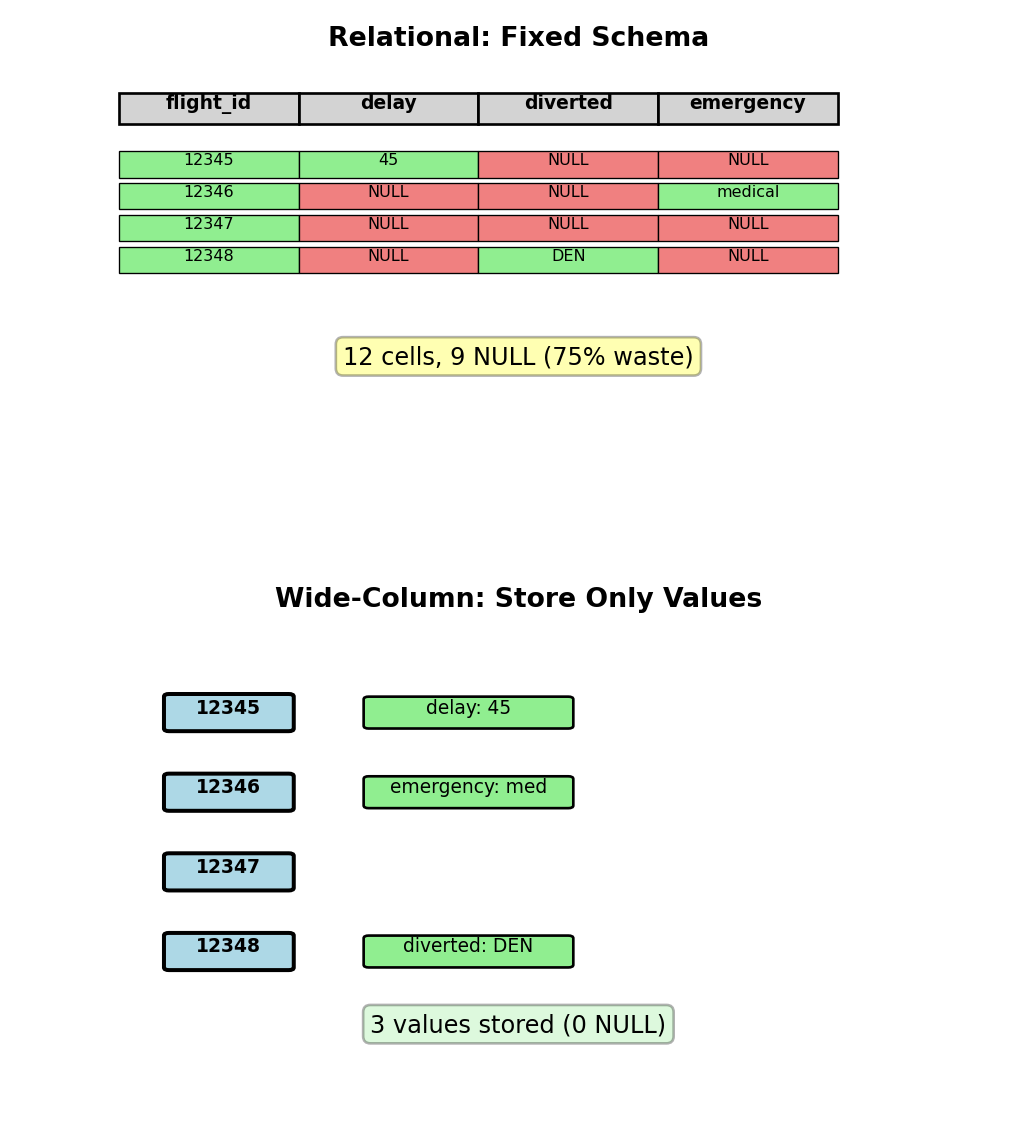

Column families provide structure, columns provide flexibility

Time-Series Data - Natural Fit for Wide-Column

Scenario: Server monitoring metrics

10,000 servers
Metrics every 10 seconds: CPU, memory, disk I/O, network
Sparse: I/O metrics only when disk active (~30% of time)
Retention: 90 days

Data volume:

10,000 servers × 6 samples/minute = 60,000 writes/minute
86.4M samples/day
90 days = 7.78B samples

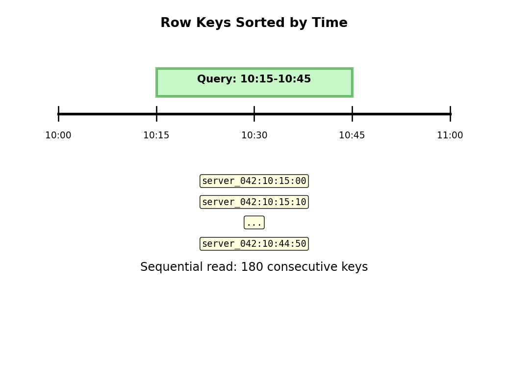
Row key design: server_id:timestamp

server_042:2025-01-15T10:30:00
server_042:2025-01-15T10:30:10
server_042:2025-01-15T10:30:20

Lexicographic sort → time-adjacent data stored adjacently

Query: “Server 42, last hour”

Start: server_042:2025-01-15T09:30:00
End:   server_042:2025-01-15T10:30:00

Sequential read of 360 consecutive row keys

Column families:

system: cpu_percent=45.2, memory_mb=8192, uptime_sec=345600
disk:   read_iops=120, write_iops=80, queue_depth=3
        (only when disk active)
network: rx_bytes=1048576, tx_bytes=524288, connections=42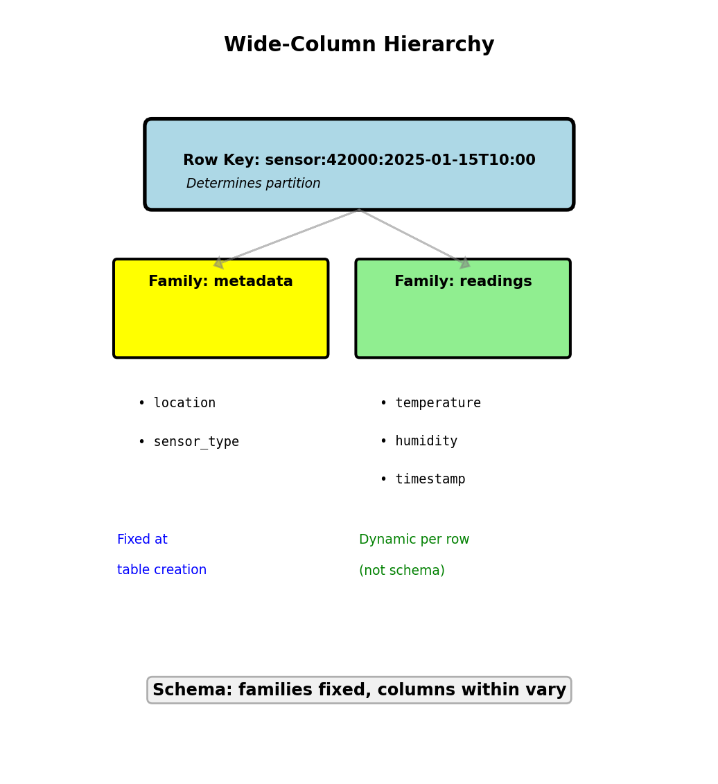

Time-ordered row keys enable efficient range queries

Storage efficiency (1M samples): Relational with NULLs: 1000 MB, Wide-Column sparse: 400 MB (60% reduction)

Cassandra Architecture - Distributed by Design

Peer-to-peer: All nodes equal

No primary-replica distinction
Any node can handle any request
Consistent hashing distributes row keys

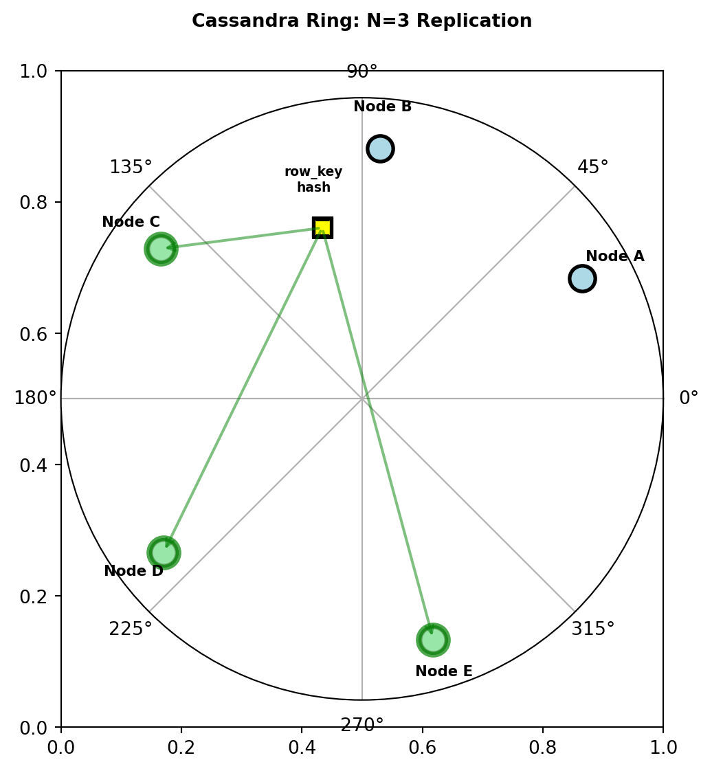
Partitioning:

Row key hashed to token (0 to 2^63-1)
Token ring: Nodes own token ranges
Replication factor N=3: Each row stored on 3 nodes

Write path:

Client sends write to any node (coordinator)
Coordinator determines replicas from hash(row_key)
Write sent to N=3 replica nodes
Coordinator waits based on consistency level:
- ONE: Wait for 1 acknowledgment (5ms)
- QUORUM: Wait for 2 of 3 (10ms, parallel writes)
- ALL: Wait for all 3 (30ms)

Write durability on each node:

Write arrives
  ↓
Commit log (sequential append, durable)
  ↓
Memtable (in-memory, fast)
  ↓
[Background: Flush memtable → SSTable on disk]

Commit log ensures no data loss if node crashes

Read path:

Query replicas (number based on consistency)
If replicas disagree: Return latest (by timestamp)
Background read repair reconciles replicas

Hash determines primary node, N consecutive nodes store replicas

Compound Primary Key - Partition and Clustering

Primary key = (partition key, clustering columns)

Partition key: Determines node placement (hash distribution)

Clustering columns: Sort order within partition (range queries)

Table definition:

CREATE TABLE sensor_readings (
    sensor_id INT,
    timestamp TIMESTAMP,
    temperature FLOAT,
    humidity FLOAT,
    PRIMARY KEY (sensor_id, timestamp)
);

sensor_id = partition key (which node)
timestamp = clustering column (sort order)

Physical layout on Node 3:

Partition: sensor_id=42000
  timestamp=2025-01-15T10:00:00, temp=22.5, humidity=45
  timestamp=2025-01-15T10:01:00, temp=22.6, humidity=46
  timestamp=2025-01-15T10:02:00, temp=22.4, humidity=45
  ... (sorted by timestamp)

Partition: sensor_id=42001
  timestamp=2025-01-15T10:00:00, temp=19.5, humidity=50
  ...

Efficient query (uses partition key + clustering):

SELECT * FROM sensor_readings
WHERE sensor_id = 42000
  AND timestamp >= '2025-01-15T10:00:00'
  AND timestamp < '2025-01-15T11:00:00';

Single node, sequential read of 60 rows

Inefficient query (missing partition key):

SELECT * FROM sensor_readings
WHERE timestamp > '2025-01-15T10:00:00';

Must query ALL nodes, scatter-gather

Query cost: O(1) partition + O(log M + K) vs O(N nodes)

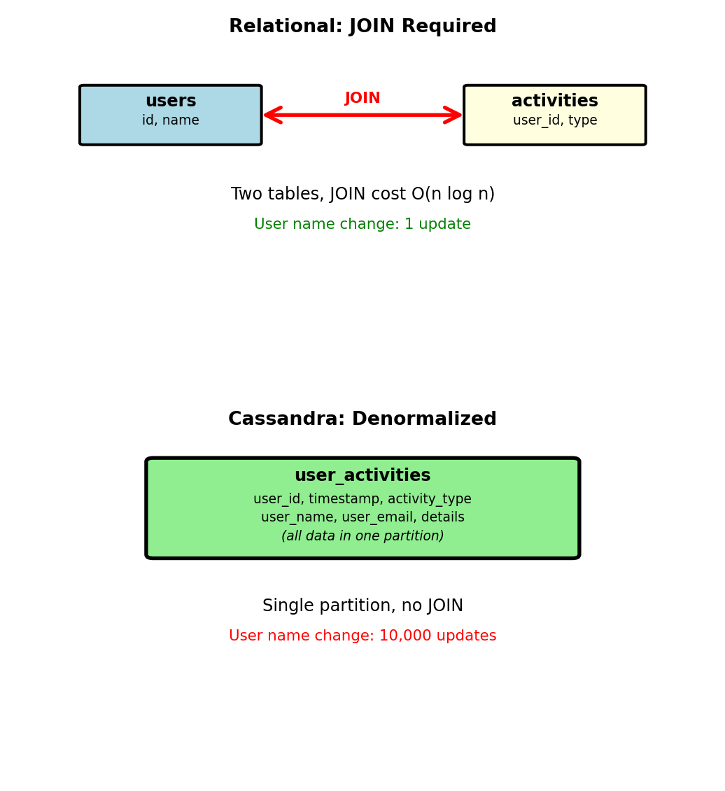
Denormalization Required - No JOINs

Cassandra has no JOIN operation

Data for query must exist in single partition

Relational approach (JOINs):

-- users table
CREATE TABLE users (
  user_id INT PRIMARY KEY,
  name VARCHAR(100),
  email VARCHAR(100)
);

-- activities table
CREATE TABLE activities (
  activity_id INT PRIMARY KEY,
  user_id INT,
  activity_type VARCHAR(50),
  timestamp TIMESTAMP,
  details TEXT
);

-- Query with JOIN
SELECT a.*, u.name
FROM activities a
JOIN users u ON a.user_id = u.user_id
WHERE a.timestamp > NOW() - INTERVAL '24 hours';

Cassandra approach (denormalized):

CREATE TABLE user_activities (
    user_id INT,
    timestamp TIMESTAMP,
    activity_type TEXT,
    user_name TEXT,     -- Denormalized
    user_email TEXT,    -- Denormalized
    details TEXT,
    PRIMARY KEY (user_id, timestamp)
) WITH CLUSTERING ORDER BY (timestamp DESC);

Query:

SELECT * FROM user_activities
WHERE user_id = 12345
  AND timestamp > '2025-01-15T00:00:00';

Single partition, no JOIN

Update cost:

User name changes → update all activity records
User with 10,000 activities: 10,000 updates
Trade-off: Query simplicity for update complexity

Acceptable when reads >> writes (activity log read 1000×, name changes rarely)

Multiple Query Patterns - Multiple Tables

Cannot optimize single table for multiple partition keys

Solution: Duplicate data in tables with different primary keys

Query pattern 1: Posts by user (timeline)

CREATE TABLE posts_by_user (
    user_id INT,
    post_timestamp TIMESTAMP,
    post_id UUID,
    content TEXT,
    likes INT,
    PRIMARY KEY (user_id, post_timestamp)
) WITH CLUSTERING ORDER BY (post_timestamp DESC);

-- Efficient: Single partition
SELECT * FROM posts_by_user
WHERE user_id = 12345
LIMIT 20;

Query pattern 2: Posts by tag (search)

CREATE TABLE posts_by_tag (
    tag TEXT,
    post_timestamp TIMESTAMP,
    post_id UUID,
    user_id INT,      -- Duplicated
    content TEXT,     -- Duplicated
    likes INT,        -- Duplicated
    PRIMARY KEY (tag, post_timestamp)
) WITH CLUSTERING ORDER BY (post_timestamp DESC);

-- Efficient: Single partition
SELECT * FROM posts_by_tag
WHERE tag = 'nosql'
LIMIT 20;

Write path:

Application writes to both tables
Post with 5 tags: 1 write to posts_by_user + 5 writes to posts_by_tag
Total: 6 writes for 1 post

Storage: 6× duplication for 5-tag post

Trade: Storage and write complexity for query performance

TTL - Automatic Data Expiration

Time-series data has natural lifecycle

Old data less valuable, must be removed

Manual deletion: Expensive

DELETE FROM sensor_readings
WHERE timestamp < '2025-01-15' - INTERVAL '90 days';

Scans entire table, expensive on billions of rows

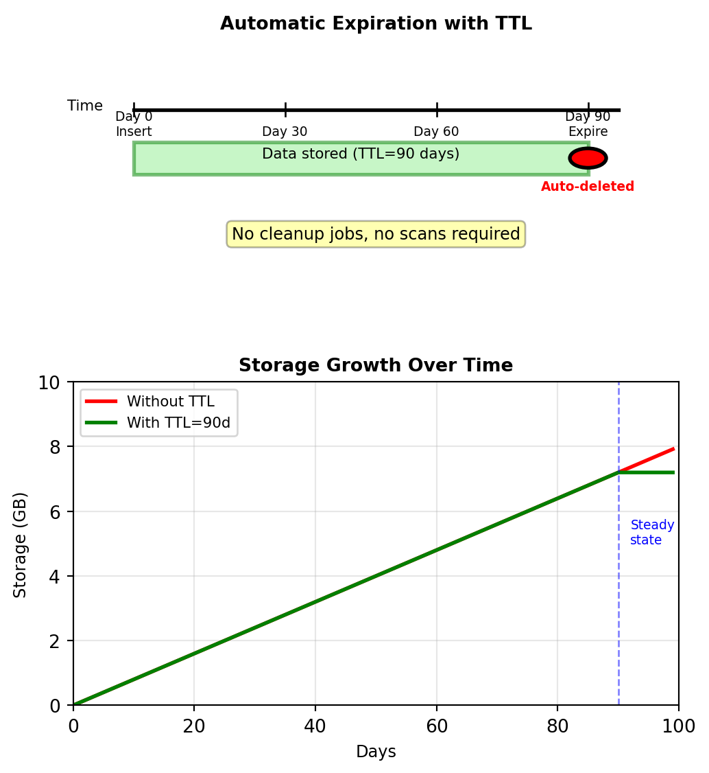
TTL (time to live): Automatic expiration

INSERT INTO sensor_readings
  (sensor_id, timestamp, temperature, humidity)
VALUES (42000, '2025-01-15T10:00:00', 22.5, 45)
USING TTL 7776000;  -- 90 days in seconds

-- After 90 days: Row automatically deleted

Implementation:

TTL stored as metadata with each column
Compaction removes expired data during background merge
Tombstone created at expiration (soft delete)
No read-time overhead: Expired data not returned

Use cases:

Monitoring data: 90-day retention
Session data: 30-minute expiration
Cache data: 5-minute expiration
Rate limiting counters: Hourly expiration

Storage calculation:

10,000 sensors × 8,640 readings/day = 86.4M rows/day
Without TTL: Unbounded growth
With 90-day TTL: Steady state at 7.78B rows

Graph Databases

Graph Model - Nodes, Edges, Properties

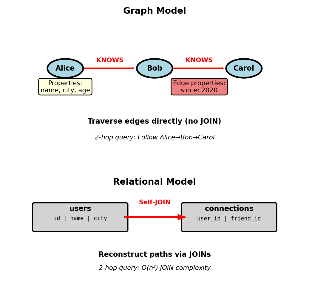
Social network queries require expensive self-JOINs:

-- Friends-of-friends
SELECT DISTINCT u.name
FROM connections c1
  JOIN connections c2 ON c1.friend_id = c2.user_id
  JOIN users u ON c2.friend_id = u.id
WHERE c1.user_id = 123;

Graph model stores relationships directly:

Nodes: Entities with properties
Edges: Relationships between nodes, can have properties
Query: Traverse edges, no JOIN operations

Example:

Node: Person {id: 123, name: “Alice”, city: “Boston”}
Edge: (Alice)-[:KNOWS {since: 2020}]->(Bob)
Query “friends of friends” = follow 2 edges

Native graph databases store adjacency (pointers between nodes), not foreign keys

Path Traversal - Friends of Friends in Neo4j

Query: Find friends-of-friends who live in Boston

Cypher (Neo4j query language):

MATCH (me:Person {id: 123})-[:KNOWS]->(friend)
      -[:KNOWS]->(fof:Person)
WHERE fof.city = 'Boston'
  AND fof.id <> 123
RETURN fof.name, fof.city

Pattern matching: (node)-[edge]->(node) describes path structure

Relational equivalent:

SELECT DISTINCT u.name, u.city
FROM connections c1
  JOIN connections c2 ON c1.friend_id = c2.user_id
  JOIN users u ON c2.friend_id = u.id
WHERE c1.user_id = 123
  AND u.city = 'Boston'
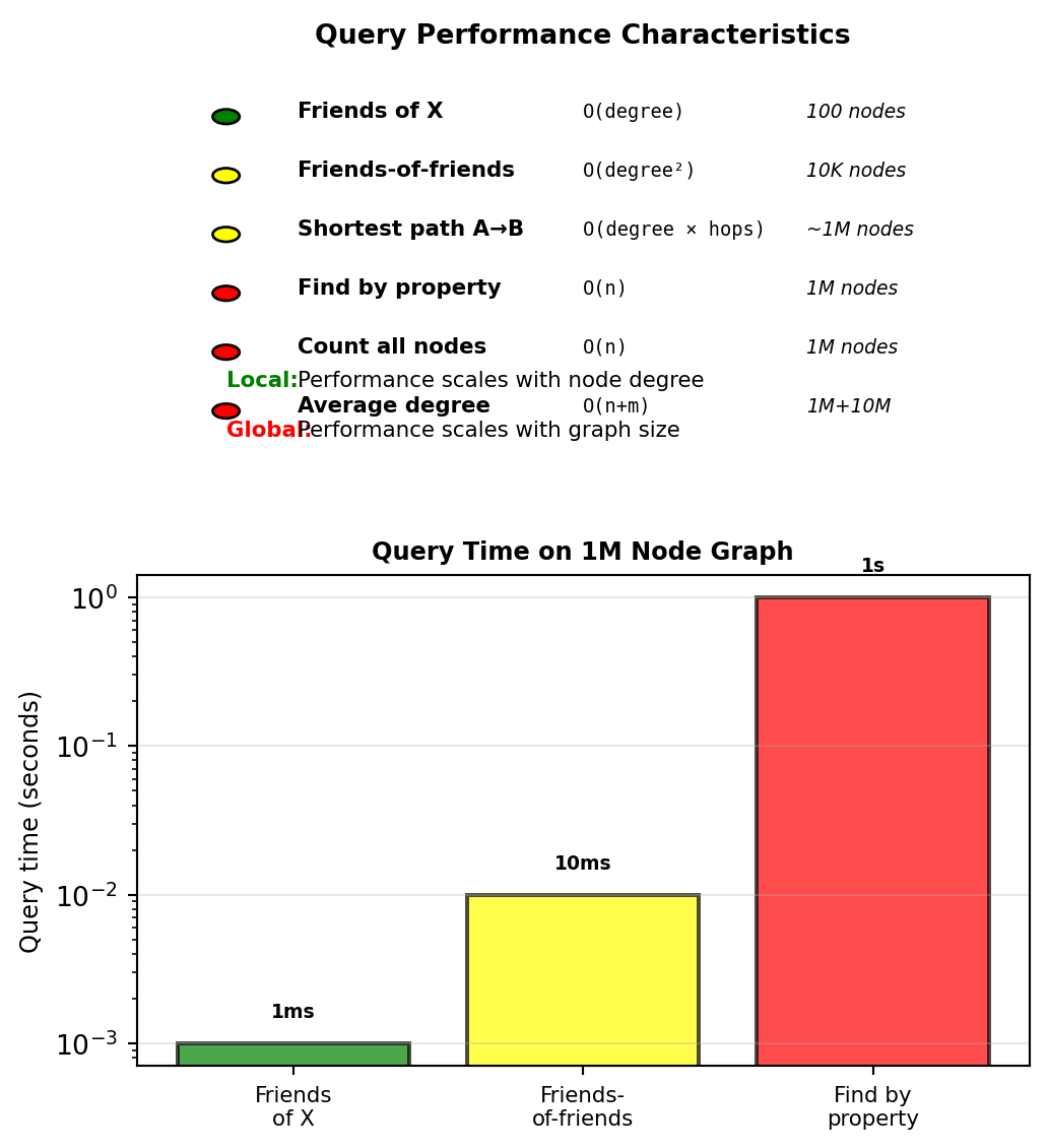
  AND c2.friend_id <> 123;

Performance difference:

Relational: O(n²) - must JOIN entire connections table twice
Graph: O(degree²) - follows edges from specific node

For node with 100 friends, each friend has 100 friends:

Graph: Explores ~10,000 nodes
SQL: Must process millions of rows (even with indexes)

Graph complexity depends on local structure (node degree), not global table size

Variable-Length Paths - Connection Distance

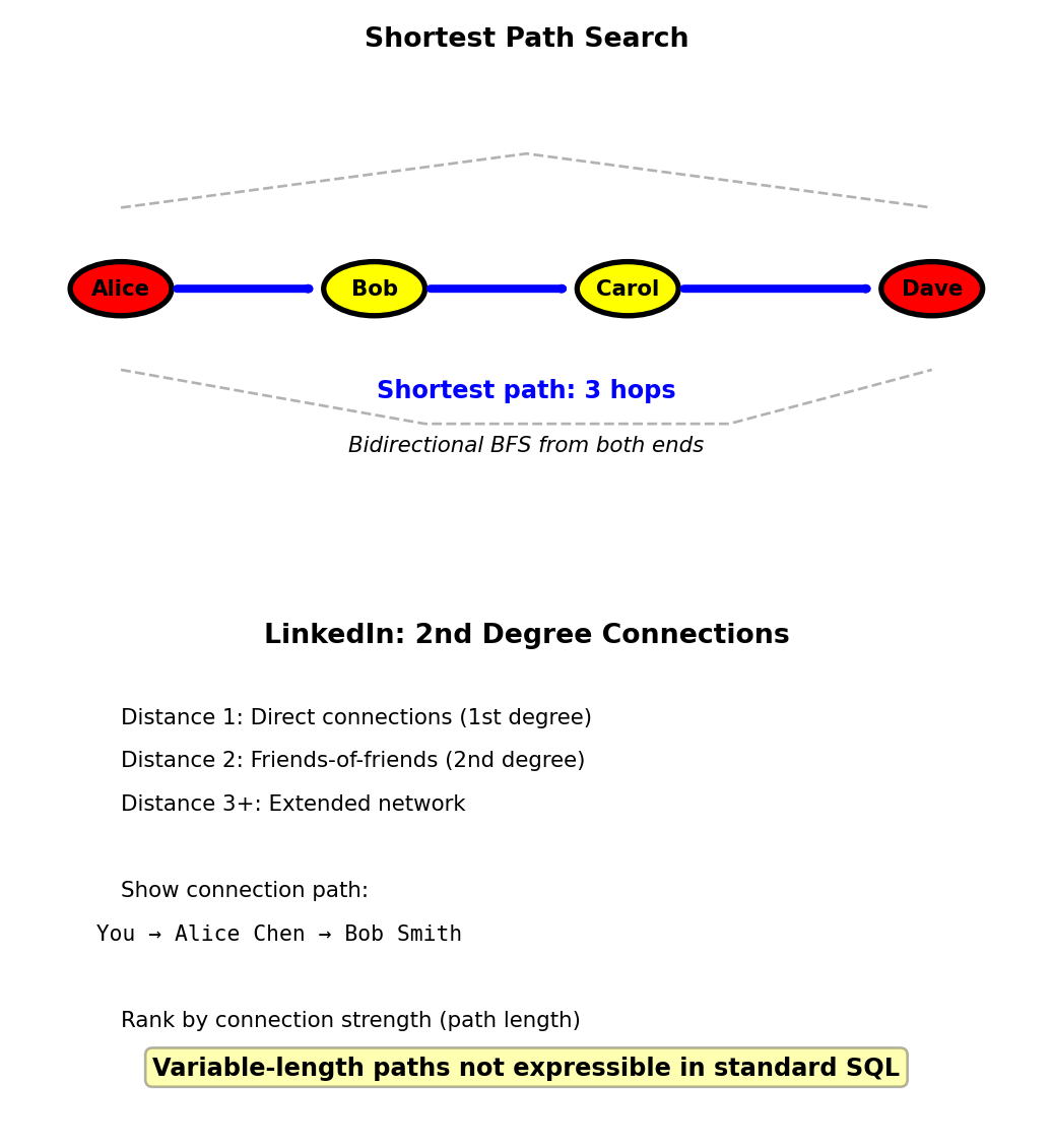
Query: How many hops separate two people? Find shortest path.

Cypher:

MATCH path = shortestPath(
  (a:Person {id: 123})-[:KNOWS*]-(b:Person {id: 789})
)
RETURN length(path)

[:KNOWS*] matches 1 or more KNOWS edges
Finds shortest connection: 2 hops, 3 hops, etc.
Bidirectional breadth-first search from both ends

Return path details:

RETURN [node IN nodes(path) | node.name] AS connection_path
-- Result: ["Alice", "Bob", "Carol", "Dave"]

SQL equivalent:

Requires recursive CTE (PostgreSQL, Oracle)
Limited depth, complex syntax
Poor performance on large graphs

WITH RECURSIVE paths AS (
  SELECT user_id, friend_id, 1 AS depth,
         ARRAY[user_id, friend_id] AS path
  FROM connections
  WHERE user_id = 123
  UNION ALL
  SELECT p.user_id, c.friend_id, p.depth + 1,
         p.path || c.friend_id
  FROM paths p
  JOIN connections c ON p.friend_id = c.user_id
  WHERE p.depth < 6
    AND NOT c.friend_id = ANY(p.path)
)
SELECT MIN(depth) FROM paths WHERE friend_id = 789;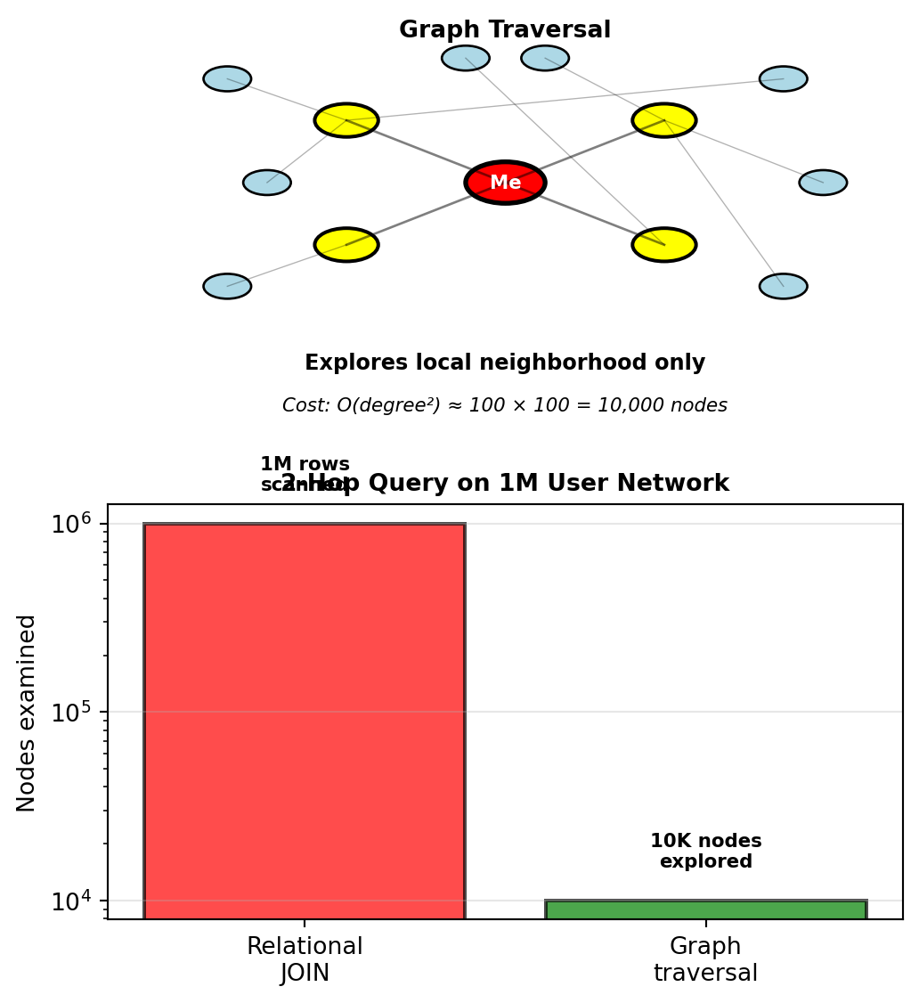

Use case: LinkedIn shows connection path and degree of separation

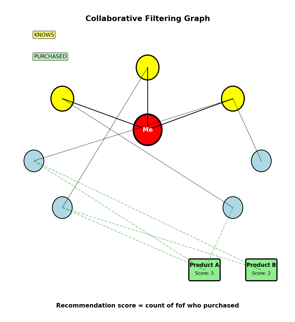
Recommendation - Collaborative Filtering

Problem: Recommend products based on friend purchases

Query: Products bought by friends-of-friends but not by me or my direct friends

MATCH (me:Person {id: 123})-[:KNOWS*1..2]->(friend)
MATCH (friend)-[:PURCHASED]->(product:Product)
WHERE NOT (me)-[:PURCHASED]->(product)
  AND NOT (me)-[:KNOWS]->()-[:PURCHASED]->(product)
RETURN product.name, COUNT(friend) as recommendation_score
ORDER BY recommendation_score DESC
LIMIT 10

Query breakdown:

[:KNOWS*1..2] = 1 or 2 hops (friends + friends-of-friends)
Find products purchased by anyone in that set
Filter out: products I’ve bought
Filter out: products my direct friends bought
Count recommendations from multiple sources

Performance:

Traverses ~10,000 relationships (100 friends × 100 fof)
Filters and aggregates during traversal
Returns top 10 products
Completes in ~50ms

Relational equivalent:

3 self-JOINs on connections table
JOIN with purchases table
Multiple subqueries for filtering
Scans millions of rows
Completes in ~5 seconds

Results:

Product A: 3 friends-of-friends purchased → score 3
Product B: 2 friends-of-friends purchased → score 2

Relational requires 3 self-JOINs + product JOIN + filtering subqueries

Knowledge Graphs - Multi-Type Relationships

Movie database with heterogeneous relationships:

Schema (property graph model):

Nodes:
  Person (name, birth_year)
  Movie (title, year, rating)
  Genre (name)

Edges:
  (Person)-[:ACTED_IN {role: "Batman"}]->(Movie)
  (Person)-[:DIRECTED]->(Movie)
  (Movie)-[:BELONGS_TO_GENRE]->(Genre)

Query: Actors who worked with directors who directed Sci-Fi movies

MATCH (actor:Person)-[:ACTED_IN]->(m1:Movie)
  <-[:DIRECTED]-(director:Person)
MATCH (director)-[:DIRECTED]->(m2:Movie)
  -[:BELONGS_TO_GENRE]->(g:Genre {name: 'Sci-Fi'})
WHERE m1 <> m2
RETURN DISTINCT actor.name, director.name, m2.title

Query breakdown:

Find actor-director collaborations
Find other movies directed by same director
Filter for Sci-Fi genre
Different relationship types (ACTED_IN, DIRECTED, BELONGS_TO_GENRE)

Relational equivalent:

5 tables: people, movies, genres, movie_actors, movie_directors, movie_genres
4 JOINs with filtering on relationship types
Complex foreign key navigation

Heterogeneous graphs: Multiple node types, multiple edge types with different semantics

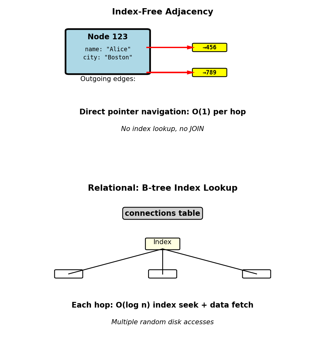
Property Graph Storage - Index-Free Adjacency

Native graph databases store direct pointers between nodes:

Conceptual storage structure:

Node 123 (Alice):
  properties: {name: "Alice", city: "Boston"}
  outgoing_edges: [ptr→456, ptr→789]
  incoming_edges: [ptr→234]

Node 456 (Bob):
  properties: {name: "Bob", city: "NYC"}
  outgoing_edges: [ptr→123, ptr→999]
  incoming_edges: [ptr→123, ptr→555]

Traversal cost:

Follow edge: O(1) pointer dereference
No index lookup required
No JOIN operation
Cache-efficient: Related nodes stored nearby on disk

Relational comparison:

JOIN requires: Index lookup O(log n) or table scan O(n)
Even with B-tree indexes: Multiple random disk seeks
Each hop: Seek to index, seek to data
Graph: Sequential read following pointers

Physical layout:

Nodes clustered by locality
Edges stored with source node
Adjacency list per node
Disk reads proportional to result size, not table size

Graph databases optimize for traversal, relational optimizes for joins

Graph Query Complexity - Local vs Global

Fast queries (local traversal):

Performance independent of graph size, depends on local structure:

“Friends of person X”: O(degree)
- Node with 100 friends: examine 100 nodes
- Graph size irrelevant
“Friends-of-friends of X”: O(degree²)
- 100 friends, each with 100 friends: examine 10,000 nodes
- Still independent of total graph size
“Shortest path between A and B”: O(degree × hops)
- 6 degrees of separation: explore ~1,000,000 nodes
- But only if path exists

Slow queries (global aggregation):

Must scan entire graph:

“Count all nodes”: O(n)
“Find all nodes with city = ‘Boston’”: O(n) without index
“Average node degree”: O(n + m) where m = edges

Performance example (1M node graph):

“Friends of Alice”: Examines 100 nodes (0.01% of graph)
“All people named Alice”: Examines 1M nodes (100% of graph)

When to use graph databases:

Relationship queries dominate workload
Traversal depth varies (1-6 hops)
Local neighborhood matters more than global statistics

Graph databases excel at local traversal, not global aggregation

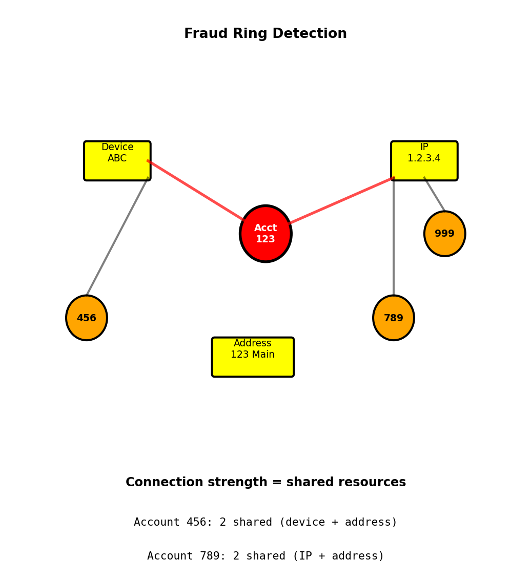
Fraud Detection - Connected Account Rings

Scenario: Credit card fraud detection - identify accounts sharing resources

Data model:

Nodes:
  Account (account_id, status)
  Device (device_fingerprint)
  IPAddress (ip)
  PhysicalAddress (street, city)

Edges:
  (Account)-[:USED_DEVICE]->(Device)
  (Account)-[:ORIGINATED_FROM]->(IPAddress)
  (Account)-[:REGISTERED_AT]->(PhysicalAddress)

Fraud detection query:

Find accounts connected to flagged account through shared resources (2 hops):

MATCH (suspicious:Account {flagged: true})
MATCH (suspicious)-[:USED_DEVICE|ORIGINATED_FROM
                    |REGISTERED_AT*1..2]-(related:Account)
WHERE related.account_id <> suspicious.account_id
RETURN related.account_id,
       COUNT(*) as connection_strength
ORDER BY connection_strength DESC

Pattern detected:

Suspicious account shares device with 3 accounts
Those 3 accounts all share same IP address
Flag entire ring for review

Timing:

Graph: 50ms to explore 2-hop neighborhood
Relational: 5s for equivalent multi-JOIN query

Relational approach:

7 tables: accounts, devices, account_devices, ips, account_ips, addresses, account_addresses
Complex multi-JOIN to find shared resources
Adding new connection type requires schema change

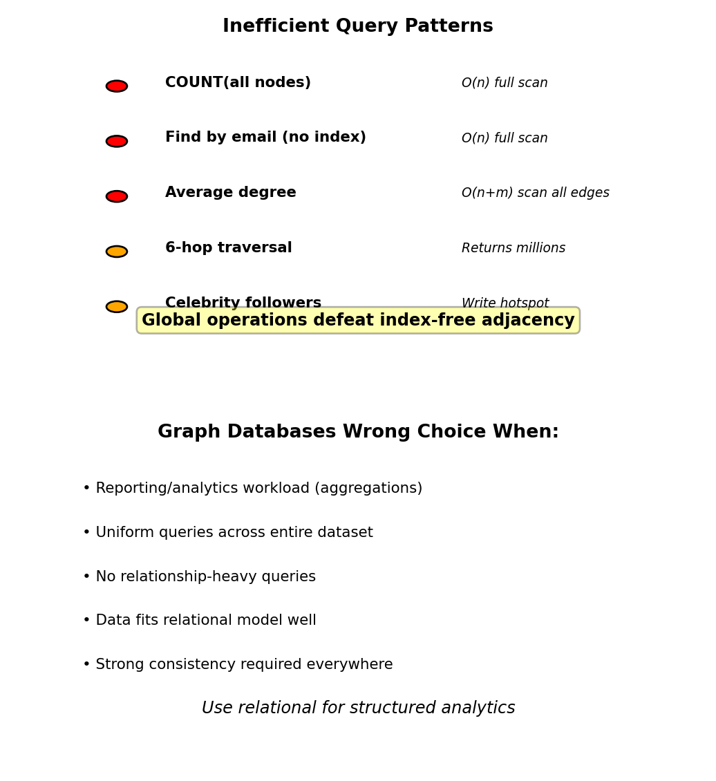
Graph Database Limitations

Inefficient without indexes:

Global aggregations require full graph scan:

// Count all users - O(n)
MATCH (u:User) RETURN COUNT(u)

// Average friend count - O(n + m)
MATCH (u:User)-[:KNOWS]->(f)
RETURN AVG(COUNT(f))

// Find by property without index - O(n)
MATCH (u:User {email: 'alice@example.com'})
RETURN u

Without property index: scans all User nodes

Large traversal results:

Small world problem - 6 degrees reaches most of graph:

// All people within 6 hops - returns millions
MATCH (me:User {id: 123})-[:KNOWS*1..6]-(connected)
RETURN COUNT(DISTINCT connected)

Kevin Bacon number: 6 hops connects to entire Hollywood

Limited transactions:

Neo4j: Full ACID transactions supported
Distributed graphs (JanusGraph, Neptune): Eventually consistent
Cross-partition transactions limited

Write hotspots:

Celebrity node with 10M followers:

Every follower edge stored on celebrity node
Hot spot for writes and reads
Sharding difficult - high-degree nodes don’t partition well

Graph databases optimize for relationship traversal, not aggregation

Polyglot Persistence

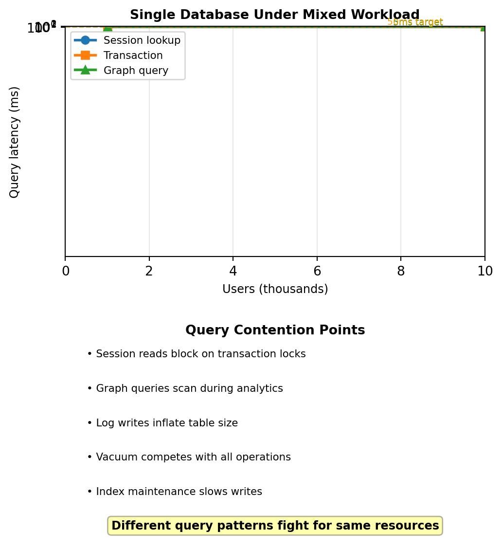
Single Database Assumption Breaks Under Heterogeneous Workload

Traditional architecture: Single PostgreSQL database

Handles everything:

User accounts, transactions, sessions
Social connections, recommendations
Logs, analytics queries

Works at small scale (thousands of users)

Observed failure at 100K users:

Session lookups (10K req/sec) compete with order writes (100 req/sec)
Friends-of-friends graph queries lock tables during analytics scans
Log inserts (1M/day) bloat primary database
Index maintenance slows all operations

Not a scale problem - a workload mismatch problem:

Shopping cart read: Needs <5ms latency, key-value lookup
Order write: Needs ACID transaction, relational integrity
Product recommendation: Needs graph traversal, relationship queries
Analytics query: Scans entire order history, full table aggregation

PostgreSQL optimized for transactions, not for all four patterns simultaneously

Query patterns interfere when forced through single storage model

E-commerce Platform - Data Flow Across Stores

Production system: 500K users, 50K orders/day

User completes checkout:

PostgreSQL (ACID transaction):

BEGIN;
  INSERT INTO orders (order_id, user_id, total, timestamp)
  VALUES (12345, 789, 99.99, NOW());

  INSERT INTO order_items (order_id, product_id, quantity, price)
  VALUES (12345, 101, 2, 49.99);

  UPDATE products SET inventory = inventory - 2
  WHERE product_id = 101 AND inventory >= 2;

  -- If inventory check fails, entire transaction rolls back
COMMIT;

Latency: 50ms | Consistency: Immediate (ACID)

Redis (ephemeral data):

# Clear shopping cart (no longer needed)
redis.delete(f"cart:{user_id}")

Latency: 1ms | Consistency: Immediate (single key)

Neo4j (graph relationship - async):

// Seconds later, from background worker
MATCH (u:User {id: 789}), (p:Product {id: 101})
CREATE (u)-[:PURCHASED {timestamp: 1234567890}]->(p)

Latency: 20ms | Consistency: Eventual (5 second delay acceptable)

Application routes operations to appropriate database

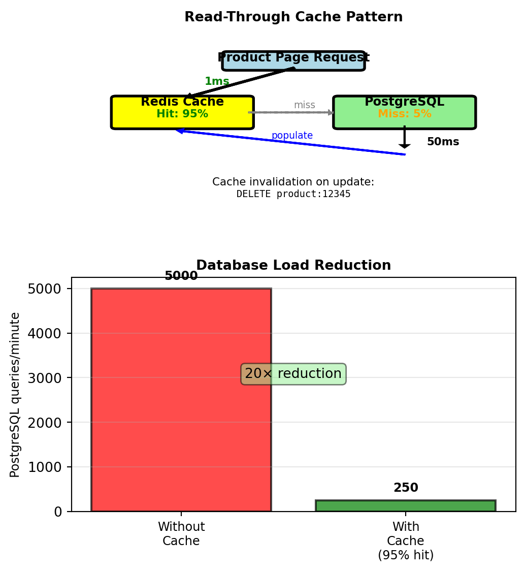
Caching Layer Reduces Primary Database Load

Problem: Product pages receive 5K views/minute

Each view queries PostgreSQL:

SELECT p.name, p.price, p.inventory,
       c.name as category,
       array_agg(i.url) as images
FROM products p
  JOIN categories c ON p.category_id = c.id
  JOIN product_images i ON p.id = i.product_id
WHERE p.id = 12345
GROUP BY p.id, c.name;

Load: 5K queries/minute = 83 queries/second to PostgreSQL

Product data changes rarely (once per day)

Read-through cache pattern:

def get_product_details(product_id):
    cache_key = f"product:{product_id}"

    cached = redis.get(cache_key)
    if cached:
        return json.loads(cached)  # 1ms cache hit

    # Cache miss - query database
    product = postgres.query(query_string, product_id)  # 50ms

    # Cache for 1 hour
    redis.setex(cache_key, 3600, json.dumps(product))
    return product

Measured performance:

Cache hit rate: 95%
Average latency: 0.95 × 1ms + 0.05 × 50ms = 3.45ms
PostgreSQL load: 5K × 0.05 = 250 queries/minute
Database load reduced 20×

Analytics queries run on read replica:

Revenue reports scan millions of rows
Run on replica: Primary unaffected
Replica lags 5-10 seconds (acceptable for reports)

Data Synchronization Without Distributed Transactions

Problem: User changes email address

Must update:

PostgreSQL users table (primary copy)
Neo4j User node (has email property for queries)

No distributed transaction across databases

Approach 1: Dual write

def update_email(user_id, new_email):
    # PostgreSQL first (source of truth)
    postgres.execute(
        "UPDATE users SET email=? WHERE id=?",
        new_email, user_id
    )

    # Neo4j second
    try:
        neo4j.run(
            "MATCH (u:User {id: $uid}) SET u.email = $email",
            uid=user_id, email=new_email
        )
    except Exception as e:
        log.error(f"Neo4j update failed: {e}")
        retry_queue.push({
            "user_id": user_id,
            "email": new_email
        })

Failure scenario:

PostgreSQL succeeds at t=0
Neo4j fails (network partition)
Retry succeeds at t=5
Neo4j shows stale email for 5 seconds
Acceptable for social graph queries

Approach 2: Event stream

# Application writes to PostgreSQL only
def update_email(user_id, new_email):
    postgres.execute("UPDATE users SET email=? WHERE id=?")
    kafka.publish("user.updated", {
        "user_id": user_id, "email": new_email
    })

# Separate consumer updates Neo4j
for event in kafka.consume("user.updated"):
    neo4j.run("MATCH (u:User {id: $uid}) SET u.email = $email")

Operational complexity:

Monitor: PostgreSQL metrics ≠ Redis metrics ≠ Neo4j metrics
Backups: Each database independent
Upgrades: PostgreSQL 14→15, Redis 6→7 separately

Polyglot Persistence in Production Architecture

Social e-commerce platform: 500K users, 50K orders/day

PostgreSQL (ACID transactions):

Tables: users, orders, order_items, products, inventory
Write: INSERT orders, UPDATE inventory atomically
Read: Point lookups by ID (indexed)
Query latency: 50ms (JOIN queries)
Load: 500 transactions/minute
Consistency: Immediate (ACID guarantees)

Redis (ephemeral cache):

Data: sessions, shopping carts, product cache
Write: SET with TTL, DELETE on invalidation
Read: GET by exact key
Query latency: 1ms
Load: 10K requests/second
Consistency: Single-key immediate

Neo4j (graph traversal):

Data: (User)-[:KNOWS]->(User), (User)-[:PURCHASED]->(Product)
Write: CREATE edge (async from PostgreSQL)
Read: MATCH paths, 2-3 hop traversal
Query latency: 20ms (friends-of-friends)
Load: 100 traversals/minute
Consistency: Eventual (5 second lag acceptable)

PostgreSQL read replica (analytics):

Same data as primary
Replication lag: 5-10 seconds
Query: Full table scans, aggregations
Query latency: 30 seconds (acceptable for reports)
Load: 10 reports/hour

Trade-off measured:

Performance: 3.45ms average page load
vs 200ms with single PostgreSQL
Complexity: 4 systems to operate
Team: Managed services or in-house expertise

Migration pattern observed:

Start: Single PostgreSQL
Pain: Session queries block transactions
Add: Redis for sessions (quick win)
Later: Neo4j for recommendations (higher value justifies complexity)

Not about database choice - about workload isolation

DynamoDB - Managed Wide-Column at Scale

DynamoDB - AWS Implementation of Wide-Column Model

DynamoDB: AWS managed database service that follows wide-column data model

Amazon’s fully managed database service:

No cluster management (contrast with Cassandra 5-node setup)
Automatic scaling based on traffic
Built-in multi-region replication
Pay-per-request pricing: $1.25 per million reads, $6.25 per million writes

Production usage:

Amazon.com: Shopping cart (50M requests/sec peak)
Lyft: Trip and location data
Snapchat: User stories storage

Trade-off vs Cassandra:

Managed service abstracts distribution complexity
Limited query flexibility (no custom partition strategies)
Operational simplicity for query constraints

Cassandra: Operator manages cluster. DynamoDB: AWS manages distribution.

Table Structure - Partition Key and Sort Key

Primary key structure determines data distribution and query patterns

Partition key (required):

Hash determines which partition stores item
Same concept as Cassandra partition key
Distribution: hash(partition_key) mod num_partitions

Sort key (optional):

Orders items within partition
Supports range queries on sort key
Physical storage: Items sorted by sort key on disk

Composite primary key = (partition key, sort key)

Sensor monitoring table:

{
    "TableName": "sensor_readings",
    "KeySchema": [
        {"AttributeName": "sensor_id", "KeyType": "HASH"},
        {"AttributeName": "timestamp", "KeyType": "RANGE"}
    ],
    "AttributeDefinitions": [
        {"AttributeName": "sensor_id", "AttributeType": "N"},
        {"AttributeName": "timestamp", "AttributeType": "N"}
    ]
}

Items for sensor_id=42000:

{"sensor_id": 42000, "timestamp": 1704034800, "temperature": 22.5}
{"sensor_id": 42000, "timestamp": 1704034810, "temperature": 22.6}
{"sensor_id": 42000, "timestamp": 1704034820, "temperature": 22.4}

All stored in same partition, sorted by timestamp

Partition key determines storage location, sort key supports range queries

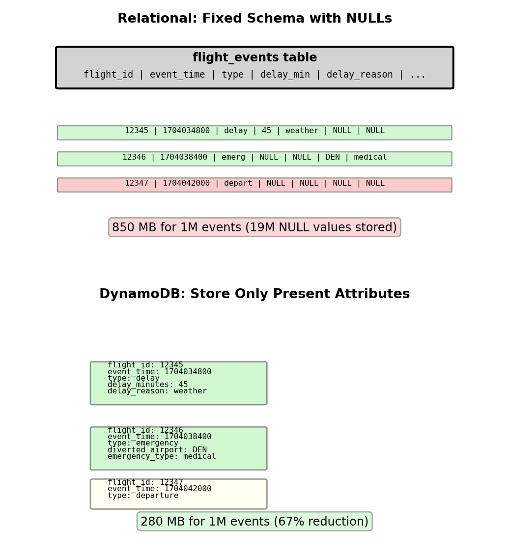
Item Structure - Sparse Storage

Items in same table can have different attributes

Wide-column stores only non-NULL values. DynamoDB implements this - no wasted storage on missing attributes.

Flight events with varying attributes:

Delay event:

{
    "flight_id": 12345,
    "event_time": 1704034800,
    "event_type": "delay",
    "delay_minutes": 45,
    "delay_reason": "weather"
}

Emergency event:

{
    "flight_id": 12346,
    "event_time": 1704038400,
    "event_type": "emergency",
    "diverted_airport": "DEN",
    "emergency_type": "medical"
}

Normal departure (no special attributes):

{
    "flight_id": 12347,
    "event_time": 1704042000,
    "event_type": "departure"
}

Storage efficiency measurement (1M flight events):

Relational approach: 20 event columns × 1M rows = 20M cells
- 95% events have no special attributes → 19M NULL values
- Storage: 850 MB (including NULL overhead)
DynamoDB: Only stores present attributes
- 50K delays (5 attributes each) + 5K emergencies (5 attributes each) + 945K normal (3 attributes each)
- Storage: 280 MB (67% reduction)

Sparse storage eliminates NULL overhead

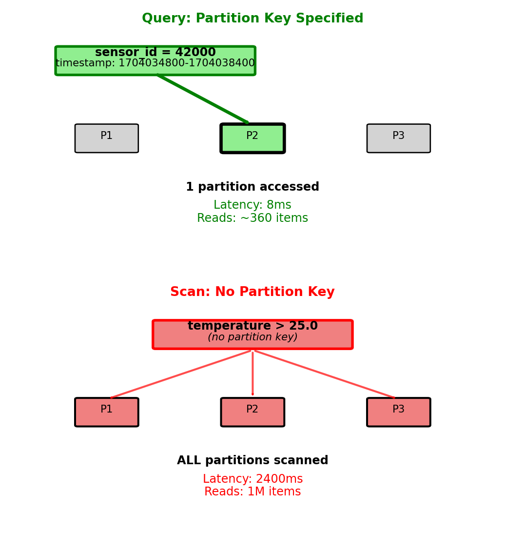
Query Patterns - Partition Key Requirement

Query performance depends on partition key specification

Like Cassandra, DynamoDB requires partition key for efficient queries. Without partition key, expensive full-table scan required.

Efficient query (partition key specified):

from boto3.dynamodb.conditions import Key

response = table.query(
    KeyConditionExpression=
        Key('sensor_id').eq(42000) &
        Key('timestamp').between(1704034800, 1704038400)
)

Execution:

Accesses single partition (sensor_id=42000)
Range scan on timestamp within partition
Returns 360 items (1 hour at 10-second intervals)
Latency: 8ms
Billed for ~360 items read

Inefficient scan (no partition key):

from boto3.dynamodb.conditions import Attr

response = table.scan(
    FilterExpression=Attr('temperature').gt(25.0)
)

Execution:

Reads every item in every partition
Applies temperature filter after reading from storage
1M total items, 100K match filter
Latency: 2400ms (300× slower)
Billed for 1M items read (not 100K returned)

Partition key specification: 300× latency difference, 2800× items read

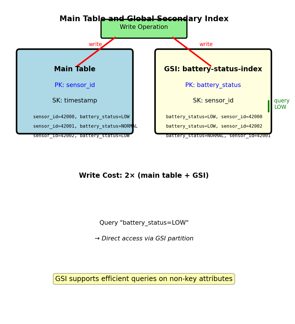
Global Secondary Index - Alternative Access Patterns

Problem: Table partitioned by sensor_id cannot efficiently query by other attributes

sensor_readings table:

Partition key: sensor_id
Sort key: timestamp
Efficient: “Readings for sensor 42000”
Inefficient: “All sensors with low battery” → requires scan

Solution: Global Secondary Index (GSI)

GSI creates alternate partition key on different attribute:

table.update(
    GlobalSecondaryIndexUpdates=[{
        'Create': {
            'IndexName': 'battery-status-index',
            'KeySchema': [
                {'AttributeName': 'battery_status', 'KeyType': 'HASH'},
                {'AttributeName': 'sensor_id', 'KeyType': 'RANGE'}
            ],
            'Projection': {'ProjectionType': 'ALL'}
        }
    }]
)

GSI structure:

New partition key: battery_status (values: LOW, NORMAL, FULL)
New sort key: sensor_id
DynamoDB maintains GSI automatically on every write

Query using GSI:

response = table.query(
    IndexName='battery-status-index',
    KeyConditionExpression=Key('battery_status').eq('LOW')
)

Returns all low-battery sensors in single partition access

GSI maintained automatically, doubles write cost

Boto3 Query Operations - Query vs Scan

Query requires partition key, scan does not

Setup:

import boto3
from boto3.dynamodb.conditions import Key, Attr

dynamodb = boto3.resource('dynamodb', region_name='us-west-2')
table = dynamodb.Table('sensor_readings')

Query with partition key and sort key range:

import time

current_time = int(time.time())
one_hour_ago = current_time - 3600

response = table.query(
    KeyConditionExpression=
        Key('sensor_id').eq(42000) &
        Key('timestamp').gt(one_hour_ago)
)

items = response['Items']
# Returns: List of items matching condition
# Example: 360 items (1 per 10 seconds for 1 hour)

Performance: Single partition access, 8ms latency

Query with additional filter (applied after retrieval):

response = table.query(
    KeyConditionExpression=Key('sensor_id').eq(42000),
    FilterExpression=Attr('temperature').gt(25.0)
)

Execution:

Reads all items for sensor_id=42000 (e.g., 10,000 items)
Filters temperature > 25.0 in memory
Returns 2,000 items (20% match filter)
Billed for 10,000 items read (not 2,000 returned)

FilterExpression reduces network transfer, not storage reads or cost

Scan entire table (avoid in production):

response = table.scan(
    FilterExpression=Attr('battery_level').lt(10)
)

items = response['Items']

Execution on 1M item table:

Reads every item in table (1M items)
Filter applied after reading from storage
Returns 50K items (5% match filter)
Latency: 3200ms
Billed for 1M items scanned

Pagination for large result sets:

items = []
last_key = None

while True:
    if last_key:
        response = table.query(
            KeyConditionExpression=Key('sensor_id').eq(42000),
            ExclusiveStartKey=last_key
        )
    else:
        response = table.query(
            KeyConditionExpression=Key('sensor_id').eq(42000)
        )

    items.extend(response['Items'])

    last_key = response.get('LastEvaluatedKey')
    if not last_key:
        break

DynamoDB returns maximum 1 MB per request. Use LastEvaluatedKey to continue.

Performance comparison (1M item table):

Query with partition key: 8ms, ~100 items read
Query with filter: 8ms, 10K items read (entire partition)
Scan: 3200ms, 1M items read (entire table)

Boto3 Item Operations

Put item (insert or replace):

table.put_item(
    Item={
        'sensor_id': 42000,
        'timestamp': 1704034800,
        'temperature': 22.5,
        'humidity': 45.0,
        'battery_level': 87
    }
)

If item with same primary key exists, replaces entirely (not merge).

Get item by primary key:

response = table.get_item(
    Key={
        'sensor_id': 42000,
        'timestamp': 1704034800
    }
)

if 'Item' in response:
    item = response['Item']
    print(f"Temperature: {item['temperature']}")
else:
    print("Item not found")

get_item returns single item, not list. Consistent read by default (can specify ConsistentRead=False for eventually consistent, half cost).

Update specific attributes:

table.update_item(
    Key={
        'sensor_id': 42000,
        'timestamp': 1704034800
    },
    UpdateExpression='SET temperature = :temp, humidity = :hum',
    ExpressionAttributeValues={
        ':temp': 23.1,
        ':hum': 46.5
    }
)

Updates only specified attributes, leaves others unchanged.

Conditional update (optimistic locking):

table.update_item(
    Key={
        'sensor_id': 42000,
        'timestamp': 1704034800
    },
    UpdateExpression='SET battery_level = :new_level',
    ConditionExpression='battery_level > :threshold',
    ExpressionAttributeValues={
        ':new_level': 85,
        ':threshold': 80
    }
)

Update succeeds only if battery_level > 80. Raises ConditionalCheckFailedException if condition false.

Delete item:

table.delete_item(
    Key={
        'sensor_id': 42000,
        'timestamp': 1704034800
    }
)

Batch operations (up to 25 items):

with table.batch_writer() as batch:
    for i in range(100):
        batch.put_item(
            Item={
                'sensor_id': 42000,
                'timestamp': 1704034800 + i * 10,
                'temperature': 22.0 + i * 0.1
            }
        )

batch_writer automatically handles batching, retries, and backoff. Reduces network round trips for bulk writes.

Cost: Same per-item cost as individual operations. Network latency reduction proportional to batch size.

AWS CLI - Table Inspection and Queries

List tables in region:

aws dynamodb list-tables --region us-west-2

Output:

{
    "TableNames": [
        "sensor_readings",
        "user_sessions",
        "flight_events"
    ]
}

Describe table structure:

aws dynamodb describe-table \
    --table-name sensor_readings \
    --region us-west-2

Returns:

KeySchema: Partition key and sort key definitions
AttributeDefinitions: Data types (N=number, S=string, B=binary)
ProvisionedThroughput or BillingMode
GlobalSecondaryIndexes: GSI definitions if present
ItemCount: Approximate item count (updated every 6 hours)
TableSizeBytes: Storage size
TableStatus: ACTIVE, CREATING, DELETING

Get specific item:

aws dynamodb get-item \
    --table-name sensor_readings \
    --key '{
        "sensor_id": {"N": "42000"},
        "timestamp": {"N": "1704034800"}
    }' \
    --region us-west-2

Note: CLI requires explicit type tags (N, S, B)

Query with CLI:

aws dynamodb query \
    --table-name sensor_readings \
    --key-condition-expression "sensor_id = :sid AND #ts > :time" \
    --expression-attribute-names '{"#ts": "timestamp"}' \
    --expression-attribute-values '{
        ":sid": {"N": "42000"},
        ":time": {"N": "1704034800"}
    }' \
    --region us-west-2

expression-attribute-names required when attribute name is reserved word (timestamp).

Output (truncated):

{
    "Items": [
        {
            "sensor_id": {"N": "42000"},
            "timestamp": {"N": "1704034810"},
            "temperature": {"N": "22.5"},
            "humidity": {"N": "45.0"}
        },
        ...
    ],
    "Count": 360,
    "ScannedCount": 360
}

Scan with filter:

aws dynamodb scan \
    --table-name sensor_readings \
    --filter-expression "battery_level < :threshold" \
    --expression-attribute-values '{":threshold": {"N": "10"}}' \
    --region us-west-2

Count: Items returned. ScannedCount: Items examined. If filter used, ScannedCount > Count (charged for ScannedCount).

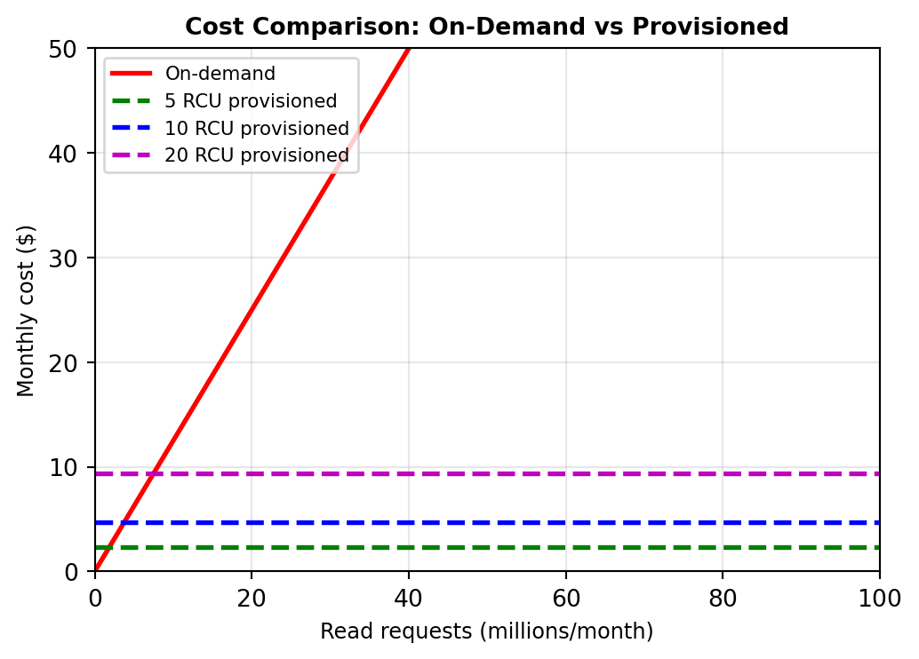
Capacity Modes - On-Demand vs Provisioned

On-demand mode: Pay per request

Pricing (us-west-2):

$1.25 per million read requests
$6.25 per million write requests
Storage: $0.25 per GB-month

Capacity unit definition:

1 read request = up to 4 KB
1 write request = up to 1 KB
Larger items consume multiple requests

Example cost calculation:

10,000 reads/day (each 2 KB) = 300K reads/month
2,000 writes/day (each 0.5 KB) = 60K writes/month
Storage: 5 GB
Monthly cost: (0.3 × $1.25) + (0.06 × $6.25) + (5 × $0.25) = $0.38 + $0.38 + $1.25 = $2.01

When to use on-demand:

Development and testing (unpredictable traffic)
Spiky workloads (traffic varies 10× between peak and baseline)
New applications (unknown traffic patterns)

Provisioned mode: Reserve capacity

Specify capacity units:

Read Capacity Units (RCU): Strongly consistent reads/sec
- 1 RCU = 1 read/sec of up to 4 KB
- Eventually consistent reads: 2× capacity (1 RCU = 2 reads/sec)
Write Capacity Units (WCU): Writes/sec of up to 1 KB

Pricing:

$0.00065/hour per RCU = $0.47/month per RCU
$0.00325/hour per WCU = $2.35/month per WCU

Provisioned capacity example:

Reserve 10 RCU + 5 WCU:

Monthly cost: (10 × $0.47) + (5 × $2.35) = $4.70 + $11.75 = $16.45
Capacity: 10 reads/sec + 5 writes/sec
Handles: 25.9M reads/month + 13M writes/month

If traffic exceeds provisioned capacity: ProvisionedThroughputExceededException (throttling). Application must retry with exponential backoff.

Auto-scaling:

table.update(
    BillingMode='PROVISIONED',
    ProvisionedThroughput={
        'ReadCapacityUnits': 10,
        'WriteCapacityUnits': 5
    }
)

# Enable auto-scaling (via AWS Application Auto Scaling)
# Target: 70% utilization
# Min: 5 RCU/WCU
# Max: 100 RCU/WCU

Auto-scaling adjusts capacity based on utilization, responds within 2-5 minutes.

Break-even analysis:

Provisioned cheaper for sustained traffic, on-demand cheaper for spiky/low-volume

DynamoDB Limitations

No server-side aggregations

Cannot compute:

# Invalid - no aggregation support
SELECT AVG(temperature) FROM sensor_readings WHERE sensor_id = 42000

Must retrieve all items and compute in application:

response = table.query(
    KeyConditionExpression=Key('sensor_id').eq(42000)
)

temperatures = [item['temperature'] for item in response['Items']]
avg_temp = sum(temperatures) / len(temperatures)

Cost: Charged for reading all items, even though only computing single aggregate value.

No joins

Cannot combine tables:

# Invalid - no JOIN support
SELECT s.*, m.location
FROM sensor_readings s
JOIN sensor_metadata m ON s.sensor_id = m.sensor_id

Must query both tables separately:

# Query 1: Get readings
readings = table_readings.query(
    KeyConditionExpression=Key('sensor_id').eq(42000)
)

# Query 2: Get metadata
metadata = table_metadata.get_item(Key={'sensor_id': 42000})

# Application joins results
for reading in readings['Items']:
    reading['location'] = metadata['Item']['location']

Alternative: Denormalize location into readings table (duplicate data, no update anomalies if location rarely changes).

Query flexibility limited

Must specify partition key:

# Invalid - no partition key
table.query(
    KeyConditionExpression=Key('timestamp').gt(1704034800)
)
# Error: Query key condition not supported

Without partition key, must use scan (reads entire table).

Item size limit: 400 KB

Cannot store:

# Invalid - item exceeds 400 KB
table.put_item(Item={
    'sensor_id': 42000,
    'timestamp': 1704034800,
    'readings': [list of 10,000 measurements]  # Too large
})

Must split large items or store in S3 with reference in DynamoDB.

Transaction limitations

TransactWriteItems supports up to 25 items:

table.meta.client.transact_write_items(
    TransactItems=[
        {'Put': {'TableName': 'sensor_readings', 'Item': {...}}},
        {'Update': {'TableName': 'sensor_metadata', 'Key': {...}, ...}},
        # ... up to 25 operations total
    ]
)

4 MB total transaction size
2× cost vs non-transactional writes
All items must be in same region

When to use relational database instead:

Complex analytical queries (aggregations, JOINs)
Ad-hoc queries (access patterns unknown at design time)
Strong multi-item consistency required across many items
Schema changes frequent

Data Modeling - Sensor Monitoring Design

Requirements:

1,000 sensors, readings every 10 seconds (100 writes/sec)
Query pattern 1: “Last hour for sensor X” (100 queries/sec)
Query pattern 2: “All sensors with temperature > 30°C” (1 query/min)
Query pattern 3: “Daily average per sensor” (batch job, 1/day)

Table design:

{
    "TableName": "sensor_readings",
    "KeySchema": [
        {"AttributeName": "sensor_id", "KeyType": "HASH"},
        {"AttributeName": "timestamp", "KeyType": "RANGE"}
    ],
    "AttributeDefinitions": [
        {"AttributeName": "sensor_id", "AttributeType": "N"},
        {"AttributeName": "timestamp", "AttributeType": "N"},
        {"AttributeName": "temp_bucket", "AttributeType": "S"}
    ],
    "GlobalSecondaryIndexes": [{
        "IndexName": "temperature-index",
        "KeySchema": [
            {"AttributeName": "temp_bucket", "KeyType": "HASH"},
            {"AttributeName": "timestamp", "KeyType": "RANGE"}
        ]
    }]
}

Rationale:

Query pattern 1 (100/sec): Partition key = sensor_id

Single partition access per query
Range on timestamp within partition (last hour = 360 items)
Latency: 8ms
Cost: 100 queries/sec × 2 RCU each = 200 RCU sustained

Query pattern 2 (1/min): GSI on temperature bucket

Partition GSI by temperature ranges: 0-10, 10-20, 20-30, 30-40
Store temp_bucket attribute: “30-40” when temperature in that range
Query GSI for temp_bucket = “30-40”
Returns all sensors in range across all partitions
Latency: 25ms, Cost: 50 RCU per query
Acceptable: 1/min × 50 RCU = 0.83 RCU sustained

Query pattern 3 (1/day): Export to S3, aggregate with Athena

DynamoDB Export to S3 (no read capacity consumed)
S3 contains Parquet files with all readings
Athena SQL query:

SELECT sensor_id,
       DATE(from_unixtime(timestamp)) as date,
       AVG(temperature) as avg_temp
FROM sensor_readings_export
GROUP BY sensor_id, DATE(from_unixtime(timestamp))

Cost: Athena query ~$0.05 per TB scanned
No DynamoDB RCU consumed

Alternative (wrong) design:

Partition key = date, Sort key = sensor_id + timestamp

{
    "partition_key": "2025-01-15",
    "sort_key": "42000#1704034800"
}

Problem: Query pattern 1 requires scanning entire day partition

1,000 sensors × 8,640 readings/day = 8.64M items per partition
Query for single sensor hour: Must scan 8.64M items to find 360
Latency: 4500ms (vs 8ms with correct design)
Cost: 8640 RCU per query (vs 2 RCU)

Design principle: Partition key must match highest-frequency query pattern. GSI handles secondary patterns at write cost increase.

Cost calculation:

Writes: 100/sec × 1 KB each = 100 WCU
Query pattern 1 reads: 200 RCU
Query pattern 2 reads: 0.83 RCU
GSI writes: 100 WCU (doubles write cost)
Total: 200 RCU + 200 WCU

Provisioned mode: (200 × $0.47) + (200 × $2.35) = $94 + $470 = $564/month

On-demand mode: 259M reads × $1.25/M + 259M writes × $6.25/M = $324 + $1619 = $1943/month

Provisioned mode 3.4× cheaper for sustained traffic.

Single-Table Design - Multiple Entities in One Table

Advanced pattern: Store multiple entity types in single table

Wide-column model supports heterogeneous rows. DynamoDB extends this - different entity types in same table using composite key structure.

Multi-table approach (relational thinking):

users_table:        PK: user_id
orders_table:       PK: order_id
products_table:     PK: product_id
order_items_table:  PK: order_id, SK: product_id

Query “user profile + recent 10 orders + line items for each order”:

Query 1: users_table → 1 item
Query 2: orders_table (GSI on user_id) → 10 items
Query 3: order_items_table (10 separate queries) → 50 items
Total: 12 requests, 45ms latency, 15 RCU

Single-table approach:

application_table:
  PK: USER#alice,      SK: PROFILE           → user data
  PK: USER#alice,      SK: ORDER#2025-01-15  → order summary
  PK: ORDER#12345,     SK: METADATA          → order details
  PK: ORDER#12345,     SK: ITEM#widget       → line item

Query “user profile + recent orders”:

table.query(
    KeyConditionExpression=Key('PK').eq('USER#alice')
)

Returns user profile + all orders in single request (11 items), 8ms latency, 3 RCU

Trade-off:

Benefit: Fewer queries (12→1), lower latency (45ms→8ms), lower cost (15→3 RCU)
Cost: Must know access patterns at design time, cannot query “all orders” efficiently (no partition key)

Single query retrieves related entities, no GSI overhead

Single-Table Design - Access Pattern Implementation

Concrete example: E-commerce order system

Table structure with composite keys encoding entity type and relationships:

User entity:

{
    "PK": "USER#alice",
    "SK": "PROFILE",
    "email": "alice@example.com",
    "name": "Alice Chen",
    "created": "2024-01-15"
}

User’s orders (sorted by date):

{
    "PK": "USER#alice",
    "SK": "ORDER#2025-01-15#12345",
    "order_id": "12345",
    "total": 125.50,
    "status": "shipped"
}

Order metadata (alternate access pattern):

{
    "PK": "ORDER#12345",
    "SK": "METADATA",
    "user_id": "alice",
    "order_date": "2025-01-15",
    "shipping_address": "123 Main St"
}

Order line items:

{
    "PK": "ORDER#12345",
    "SK": "ITEM#widget",
    "product_name": "Widget Pro",
    "quantity": 2,
    "price": 50.00
}

Access pattern 1: User profile + recent orders

response = table.query(
    KeyConditionExpression=
        Key('PK').eq('USER#alice') &
        Key('SK').begins_with('ORDER#')
)

Returns:

All orders for user (sorted by date in SK)
Single partition access
Latency: 8ms, Cost: 3 RCU (reads ~10 items)

Access pattern 2: Order details + line items

response = table.query(
    KeyConditionExpression=Key('PK').eq('ORDER#12345')
)

Returns:

METADATA item + all ITEM# items
Single partition access
Latency: 5ms, Cost: 1 RCU (reads 4 items)

Performance comparison:

Multi-table design:

Pattern 1: Query users + query orders (with GSI) = 15ms
Pattern 2: Query orders + query order_items = 12ms
GSI on orders.user_id: Doubles write cost
Total latency: 27ms

Single-table design:

Pattern 1: Single query = 8ms
Pattern 2: Single query = 5ms
No GSI required
Total latency: 13ms (52% reduction)

Sort key ordering (ORDER#2025-01-15#12345) provides chronological sorting without additional index. Latest orders retrieved first by reversing sort direction.

Constraint: Cannot efficiently query “all orders across all users” (no partition key). Single-table design optimizes for known access patterns, not ad-hoc queries.

DynamoDB in System Architecture

DynamoDB complements relational databases

PostgreSQL RDS (relational):

User accounts: id, email, password_hash, created_at
Subscription plans: plan_id, name, price_cents, features
Payment transactions: txn_id, user_id, amount, status, timestamp
Referential integrity: Foreign keys, CASCADE deletes
ACID transactions for payment processing

DynamoDB (wide-column):

User activity logs: user_id + timestamp → action, resource, metadata
API rate limiting: api_key + window_start → request_count, TTL
Session storage: session_token → user_id, login_time, expires_at
Real-time sensor data: device_id + timestamp → measurements
High write throughput, key-based access, TTL for automatic expiration

S3 (object storage):

Raw log files (archived from DynamoDB)
User-uploaded files
ML model artifacts
Static website assets

Data flow example (IoT sensor platform):

Sensor HTTP POST → API Gateway → Lambda function
Lambda writes to DynamoDB (sensor_id, timestamp, readings)
- Write latency: 5ms
- Cost: 1 WCU per reading
DynamoDB Stream triggers Lambda for anomaly detection
- Stream provides ordered change log
- Lambda processes each reading within 100ms
Anomaly detected → Lambda writes alert to PostgreSQL
- alerts table: alert_id, sensor_id, severity, timestamp, description
- Triggers notification to operations team
Nightly batch job: DynamoDB → S3 Export
- Parquet format for analytics
- Athena queries for daily/weekly aggregates
Monthly aggregates → PostgreSQL for dashboard queries

Each storage system handles workload it optimizes for